We download the precompiled data of adakite from GEOROC database. For a simple impression of adakite, the wikipedia page gives some clue: Adakites are volcanic rocks of intermediate to felsic composition that have geochemical characteristics of magma thought to have formed by partial melting of altered basalt that is subducted below volcanic arcs.
In this example, we demonstrate how to use python to simplify the data, discard the null data, classify and plot the geochemical properties.
import pandas as pd
import matplotlib.pyplot as plt
from mpl_toolkits.basemap import Basemap
import warnings
warnings.filterwarnings("ignore")
plt.rcParams['figure.figsize'] = (20, 10)
plt.style.use('default')
df = pd.read_csv("ADAKITE.csv", encoding="iso-8859-1")
df = df.dropna(axis=1, thresh=int(0.5*len(df)))
def plot_harker(x,xlabel,y,ylabel,title=None,xlim=[40,80],ylim=None,color = "b",label=None):
    plt.scatter(x=x,y=y,marker="o", c=color,s=8,label = label)
    plt.xlabel(xlabel)
    plt.ylabel(ylabel)
    plt.xlim(xlim)
    try:
        plt.ylim(ylim)
    except:
        pass
    if title != None:
        plt.title(title)
plt.figure(figsize=(10,10))
m = Basemap(lon_0=180,projection='hammer')
lon = df["LONGITUDE MIN"].dropna()
lat = df["LATITUDE MIN"].dropna()
lon = pd.to_numeric(lon, errors='ignore');
lat = pd.to_numeric(lat, errors='ignore');
lon_ = [];lat_ = []
for x, y in zip(lon,lat):
    try:
        xx, yy = m(float(x),float(y))
        lon_.append(xx);lat_.append(yy)
    except:
        pass
m.scatter(lon_, lat_, marker = "o" ,s=15, c="r" , edgecolors = "k", alpha = 1)
m.drawcoastlines()
plt.title('Adakite rocks sample')
plt.show()

plt.figure(figsize=(12,12))
plt.subplot(321)
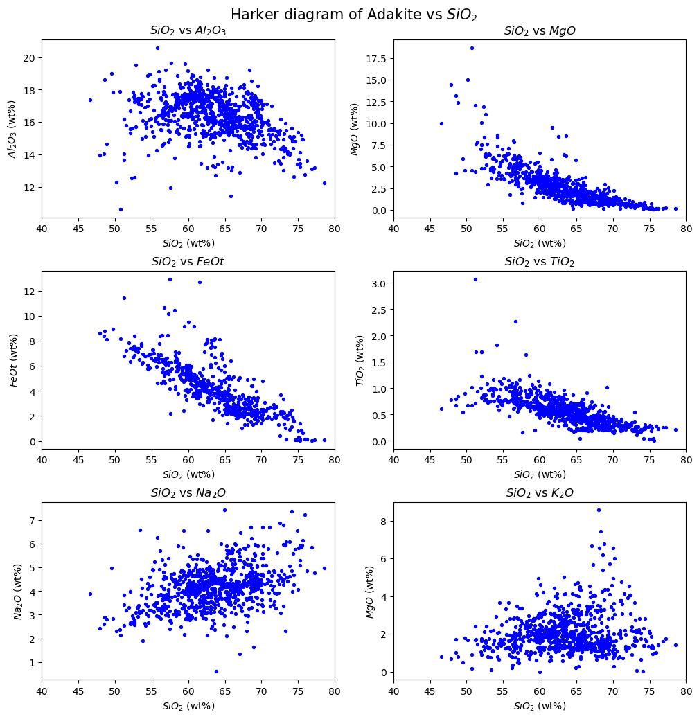
plot_harker(x=df["SIO2(WT%)"],xlabel=r'$SiO_2$ (wt%)',
y=df["AL2O3(WT%)"],ylabel=(r'$Al_2O_3$ (wt%)'),title=r'$SiO_2$ vs $Al_2O_3$')
plt.subplot(322)
plot_harker(x=df["SIO2(WT%)"],xlabel=r'$SiO_2$ (wt%)',
y=df["MGO(WT%)"],ylabel=(r'$MgO$ (wt%)'),title=r'$SiO_2$ vs $MgO$')
plt.subplot(323)
plot_harker(x=df["SIO2(WT%)"],xlabel=r'$SiO_2$ (wt%)',
y=df["FEOT(WT%)"],ylabel=(r'$FeOt$ (wt%)'),title=r'$SiO_2$ vs $FeOt$')
plt.subplot(324)
plot_harker(x=df["SIO2(WT%)"],xlabel=r'$SiO_2$ (wt%)',
y=df["TIO2(WT%)"],ylabel=(r'$TiO_2$ (wt%)'),title=r'$SiO_2$ vs $TiO_2$')
plt.subplot(325)
plot_harker(x=df["SIO2(WT%)"],xlabel=r'$SiO_2$ (wt%)',
y=df["NA2O(WT%)"],ylabel=(r'$Na_2O$ (wt%)'),title=r'$SiO_2$ vs $Na_2O$')
plt.subplot(326)
plot_harker(x=df["SIO2(WT%)"],xlabel=r'$SiO_2$ (wt%)',
y=df["K2O(WT%)"],ylabel=(r'$MgO$ (wt%)'),title=r'$SiO_2$ vs $K_2O$')
plt.suptitle(r'Harker diagram of Adakite vs $SiO_2$',y=0.92,fontsize=15)
plt.subplots_adjust(hspace=0.3)
plt.show()
plt.figure(figsize=(8,8))
tec = df['TECTONIC SETTING'].dropna()
tec = tec.replace('ARCHEAN CRATON (INCLUDING GREENSTONE BELTS)','ARCHEAN CRATON')
tec_counts = tec.value_counts()
tec_counts.plot(kind="bar",fontsize=10)
plt.title('Tectonic settings of Adakite')
plt.ylim([0,500])
plt.show()

df['SR/Y'] = (df["SR(PPM)"]/df["Y(PPM)"])
df['CAO+NA2O'] = df['CAO(WT%)'] + df['NA2O(WT%)']
df['CR/NI'] = df['CR(PPM)'] + df['NI(PPM)']
df_hsa = df[df["SIO2(WT%)"] > 60]
df_lsa = df[df["SIO2(WT%)"] < 60]
plt.figure(figsize=(12,12))
plt.subplot(221)
plot_harker(x=df_hsa["TIO2(WT%)"],xlabel=r'$TiO_2$ (%)',
            y=df_hsa["CR/NI"],ylabel=(r'$Cr/Ni$'),
            xlim=[0,2],ylim=[0,200],color="r")
plot_harker(x=df_lsa["TIO2(WT%)"],xlabel=r'$TiO_2$ (%)',
            y=df_lsa["CR/NI"],ylabel=(r'$Cr/Ni$'),
            xlim=[0,2],ylim=[0,200],color="b")
plt.subplot(222)
plot_harker(x=df_hsa["CAO+NA2O"],xlabel=r'$CaO+Na_2O$ (%)',
            y=df_hsa["SR(PPM)"],ylabel=(r'$Sr$ (ppm)'),
            xlim=[0,20],ylim=[0,3000],color="r")
plot_harker(x=df_lsa["CAO+NA2O"],xlabel=r'$CaO+Na_2O$ (%)',
            y=df_lsa["SR(PPM)"],ylabel=(r'$Sr$ (ppm)'),
            xlim=[0,20],ylim=[0,3000],color="b")
plt.subplot(223)
plot_harker(x=df_hsa["SIO2(WT%)"],xlabel=r'$SiO_2$ (%)',
            y=df_hsa["MGO(WT%)"],ylabel=(r'$MgO$ (%)'),
            xlim=[40,80],ylim=[0,10],color="r")
plot_harker(x=df_lsa["SIO2(WT%)"],xlabel=r'$SiO_2$ (%)',
            y=df_lsa["MGO(WT%)"],ylabel=(r'$MgO$ (%)'),
            xlim=[40,80],ylim=[0,10],color="b")
plt.subplot(224)
plot_harker(x=df_hsa["Y(PPM)"],xlabel=r'$Y$ (ppm)',
            y=df_hsa["SR/Y"],ylabel=(r'$Sr/Y$'),
            xlim=[0,60],ylim=[0,200],color="r",label=r"High $SiO_2$ (>60%) adakites ")
plot_harker(x=df_lsa["Y(PPM)"],xlabel=r'$Y$ (ppm)',
            y=df_lsa["SR/Y"],ylabel=(r'$Sr/Y$'),
            xlim=[0,60],ylim=[0,200],color="b",label=r"Low $SiO_2$ (<60%) adakites")
plt.suptitle(r'Harker diagram of Low vs High $SiO_2$ adakites',y=0.92,fontsize=15)
plt.legend()
plt.show()

cite = [df.CITATIONS[x] for x in range(0,len(df)) if len(df.CITATIONS[x]) > 20 and df.CITATIONS[x].count('[') < 3]
year = []
for i in range(0,len(cite)):
    year.append(int(cite[i].split('[')[2].split(']')[0]))
plt.figure(figsize=(10,10))
plt.hist(year,40,
         facecolor='green',
         edgecolor='k')
plt.title('Number of paper about adakite vs year from GEOROC database')
plt.show()

Share this post