Introduction
This post is a compilation of the exercises from Chapter 2: Data Manipulation and Simple Calculations from the book Geochemical Modelling of Igneous Processes - Principles and Recipes in R language by Vojtěch Janoušek, Jean Hervé Martin, Vojtěch Erban and Colin Farrow.
First, we load the GCDkit library.
sink("/dev/null"); suppressPackageStartupMessages(library(GCDkit)); sink();2.1. Loading and Manipulating Data
Exercise 2.1: Subsetting a numeric vector, vector operations
GCDkit contains several built-in datasets, normally needed just for correct system functioning. One of these is atomic weights, stored in the named vector mw. We will use it to show some simple vector operations.
- Display the whole vector.
mw## Ag Al Ar As Au B Ba Be
## 107.8700 26.9820 39.9480 74.9220 196.9700 10.8000 137.3300 9.0122
## Bi Br C Ca Cd Ce Cl Co
## 208.9800 79.9000 12.0100 40.0780 112.4100 140.1200 35.4000 58.9330
## Cr Cs Cu Dy Er Eu F Fe
## 51.9960 132.9100 63.5400 162.5000 167.2600 151.9600 18.9980 55.8400
## Ga Gd Ge H He Hf Hg Ho
## 69.7230 157.2000 72.6300 1.0080 4.0026 178.4000 200.5900 164.9300
## I In Ir K Kr La Li Lu
## 126.9000 114.8200 192.2200 39.0980 83.7900 138.9100 6.9000 174.9700
## Mg Mn Mo N Na Nb Nd Ne
## 24.3000 54.9380 95.9500 14.0000 22.9900 92.9060 144.2400 20.1800
## Ni O Os P Pa Pb Pd Pr
## 58.6930 15.9990 190.2000 30.9740 231.0400 207.2000 106.4200 140.9100
## Pt Rb Re Rh Ru S Sb Sc
## 195.0800 85.4680 186.2100 102.9100 101.0000 32.0000 121.7600 44.9560
## Se Si Sm Sn Sr Ta Tb Te
## 78.9700 28.0800 150.3000 118.7100 87.6200 180.9500 158.9300 127.6000
## Th Ti Tl Tm U V W Xe
## 232.0400 47.8670 204.3000 168.9300 238.0300 50.9420 183.8400 131.2900
## Y Yb Zn Zr
## 88.9060 173.0500 65.3800 91.2200What is the atomic weight of Rb?
mw['Rb']## Rb
## 85.468- What is the average value of the whole vector?
mean(mw)## [1] 104.1671- Which atoms have the atomic weight higher than 170?
names(mw)[mw>170]## [1] "Au" "Bi" "Hf" "Hg" "Ir" "Lu" "Os" "Pa" "Pb" "Pt" "Re" "Ta" "Th" "Tl" "U"
## [16] "W" "Yb"- Display the names of six lightest and six heaviest elements in the dataset.
sort(mw)[1:6]## H He Li Be B C
## 1.0080 4.0026 6.9000 9.0122 10.8000 12.0100rev(sort(mw))[1:6]## U Th Pa Bi Pb Tl
## 238.03 232.04 231.04 208.98 207.20 204.30Excercise 2.2: Loading files, matrix/data frame manipulations
The file sazava.data contains selected major- and trace-element analyses from the ~354 Ma old Sázava suite of the Central Bohemian Plutonic Complex (CBPC; Bohemian Massif, Czech Republic) (Janoušek et al. 2000, 2004).
Read analyses stored in the tab-delimited data file into a data frame WR.
Find out the names of available variables (= column names).
data(sazava)
sazava
## Intrusion Locality Petrology Outcrop
## Sa-1 Sazava Mrac bi-amph quartz diorite working quarry
## Sa-2 Sazava Mrac bi-amph quartz diorite working quarry
## Sa-3 Sazava Mrac bi-amph quartz diorite working quarry
## Sa-4 Sazava Mrac bi-amph quartz diorite working quarry
## Sa-7 Sazava Teletin bi-amph tonalite disused quarry
## SaD-1 basic Teletin bi-amph quartz diorite disused quarry
## Gbs-1 basic Pecerady px-amph gabbro disused quarry
## Gbs-20 basic Pecerady px-amph gabbro disused quarry
## Gbs-2 basic Vavretice amph-bi qtz gabbrodiorite disused quarry
## Gbs-3 basic Brtnice amph-bi qtz gabbrodiorite water supply gallery
## Po-1 Pozary Krhanice bi trondhjemite working quarry
## Po-3 Pozary Prosecnice bi trondhjemite working quarry
## Po-4 Pozary Prosecnice bi trondhjemite working quarry
## Po-5 Pozary Prosecnice bi trondhjemite working quarry
## Symbol Colour SiO2 TiO2 Al2O3 FeO Fe2O3 MnO MgO CaO Na2O K2O P2O5
## Sa-1 10 4 59.98 0.63 16.42 5.46 1.35 0.19 3.21 7.04 2.52 2.50 0.16
## Sa-2 10 4 55.17 0.71 17.00 5.26 2.66 0.16 3.67 8.22 3.36 1.70 0.17
## Sa-3 10 4 55.09 0.75 17.59 5.81 2.13 0.15 3.52 8.20 2.83 2.04 0.21
## Sa-4 10 4 50.72 0.83 17.57 7.65 2.19 0.24 5.18 9.92 2.83 1.60 0.19
## Sa-7 10 1 57.73 0.95 18.82 5.43 1.00 0.12 2.82 7.47 2.54 1.67 0.37
## SaD-1 8 1 52.90 1.35 18.23 7.24 1.47 0.16 3.89 8.55 2.76 1.45 0.26
## Gbs-1 19 1 49.63 0.76 13.34 5.69 3.22 0.17 8.59 14.64 1.67 1.07 0.10
## Gbs-20 19 1 51.72 0.67 14.17 6.43 2.44 0.16 7.47 11.44 1.97 1.38 0.14
## Gbs-2 19 1 48.84 0.34 21.64 2.74 3.28 0.13 5.11 13.75 1.78 0.83 0.04
## Gbs-3 19 1 55.80 0.80 16.98 6.22 2.79 0.25 3.16 7.22 3.07 1.45 0.20
## Po-1 1 2 62.95 0.28 20.02 1.65 0.67 0.05 0.55 6.61 3.91 1.99 0.07
## Po-3 1 2 68.30 0.28 15.29 2.12 0.40 0.04 1.77 3.76 3.63 1.95 0.07
## Po-4 1 2 71.09 0.30 15.09 2.12 0.38 0.06 0.52 3.75 3.68 1.87 0.07
## Po-5 1 2 71.42 0.30 15.04 2.41 0.47 0.05 0.52 3.67 2.58 1.79 0.07
## CO2 F S H2O_PLUS H2O. Ba Rb Sr Zr Nb Ni Co Zn Cr La
## Sa-1 0.18 NA NA 1.18 NA 1037 76 539 76 6 10 17 71 29 NA
## Sa-2 0.04 NA 0.05 1.13 0.04 582 53 540 55 10 10 23 76 60 NA
## Sa-3 0.09 0.07 0.05 1.19 0.08 NA NA NA NA NA NA NA NA NA NA
## Sa-4 0.09 NA NA 1.17 NA 388 56 472 56 5 NA 30 104 53 21.67
## Sa-7 0.13 NA 0.12 1.14 0.03 722 57 537 57 10 NA 13 50 33 20.76
## SaD-1 0.06 0.07 0.04 1.53 0.06 1017 43 430 88 10 NA 18 85 43 NA
## Gbs-1 0.04 NA 0.03 1.61 0.10 583 21 352 76 4 22 40 75 217 NA
## Gbs-20 0.05 0.09 0.36 1.36 0.11 NA NA NA NA NA NA NA NA NA NA
## Gbs-2 0.51 NA NA 1.57 NA 245 31 278 27 8 13 23 51 159 NA
## Gbs-3 0.10 NA 0.01 1.35 0.07 860 43 325 72 4 6 16 124 30 NA
## Po-1 0.35 NA NA 0.71 NA 1024 51 599 128 5 NA NA 23 15 11.56
## Po-3 NA NA NA 0.50 NA 1338 65 406 159 4 6 NA 26 32 NA
## Po-4 0.27 NA NA 0.71 NA 1284 58 430 180 6 NA 4 22 16 26.19
## Po-5 0.17 NA NA 0.46 0.02 1519 64 408 162 8 NA 4 26 121 NA
## Ce Pr Nd Sm Eu Gd Tb Dy Ho Er Tm Yb Lu Y
## Sa-1 NA NA NA NA NA NA NA NA NA NA NA NA NA 25
## Sa-2 NA NA NA NA NA NA NA NA NA NA NA NA NA 30
## Sa-3 NA NA NA NA NA NA NA NA NA NA NA NA NA 30
## Sa-4 71.78 6.94 29.71 6.24 1.50 6.09 0.92 5.80 1.03 2.80 0.43 2.88 0.43 38
## Sa-7 42.02 4.96 17.44 3.76 1.77 3.76 0.56 2.70 0.56 1.64 0.24 1.52 0.25 24
## SaD-1 NA NA NA NA NA NA NA NA NA NA NA NA NA 36
## Gbs-1 NA NA NA NA NA NA NA NA NA NA NA NA NA 20
## Gbs-20 NA NA NA NA NA NA NA NA NA NA NA NA NA 19
## Gbs-2 NA NA NA NA NA NA NA NA NA NA NA NA NA 10
## Gbs-3 NA NA NA NA NA NA NA NA NA NA NA NA NA 42
## Po-1 17.99 1.76 5.42 1.40 1.29 1.12 0.13 0.64 0.11 0.37 0.06 0.51 0.08 11
## Po-3 NA NA NA NA NA NA NA NA NA NA NA NA NA 8
## Po-4 38.95 3.92 11.48 1.78 1.05 1.35 0.16 0.80 0.14 0.50 0.09 0.61 0.10 7
## Po-5 NA NA NA NA NA NA NA NA NA NA NA NA NA 5
## Cs Ta Hf
## Sa-1 NA NA NA
## Sa-2 NA NA NA
## Sa-3 NA NA NA
## Sa-4 5.7 0.5 2.5
## Sa-7 6.6 0.6 3.6
## SaD-1 2.3 1.1 1.8
## Gbs-1 NA NA NA
## Gbs-20 NA NA NA
## Gbs-2 NA NA NA
## Gbs-3 NA NA NA
## Po-1 3.0 0.3 4.2
## Po-3 NA NA NA
## Po-4 3.0 0.2 5.4
## Po-5 NA NA NAprint(colnames(sazava))## [1] "Intrusion" "Locality" "Petrology" "Outcrop" "Symbol" "Colour"
## [7] "SiO2" "TiO2" "Al2O3" "FeO" "Fe2O3" "MnO"
## [13] "MgO" "CaO" "Na2O" "K2O" "P2O5" "CO2"
## [19] "F" "S" "H2O_PLUS" "H2O." "Ba" "Rb"
## [25] "Sr" "Zr" "Nb" "Ni" "Co" "Zn"
## [31] "Cr" "La" "Ce" "Pr" "Nd" "Sm"
## [37] "Eu" "Gd" "Tb" "Dy" "Ho" "Er"
## [43] "Tm" "Yb" "Lu" "Y" "Cs" "Ta"
## [49] "Hf"- What is the MgO content of sample Sa-1?
sazava["Sa-1","MgO"]## [1] 3.21- Show all available numeric data for samples Po-1 and Po-4.
sazava <- sazava[,-(1:6)]
sazava[c("Po-1","Po-4"),]
## SiO2 TiO2 Al2O3 FeO Fe2O3 MnO MgO CaO Na2O K2O P2O5 CO2 F S
## Po-1 62.95 0.28 20.02 1.65 0.67 0.05 0.55 6.61 3.91 1.99 0.07 0.35 NA NA
## Po-4 71.09 0.30 15.09 2.12 0.38 0.06 0.52 3.75 3.68 1.87 0.07 0.27 NA NA
## H2O_PLUS H2O. Ba Rb Sr Zr Nb Ni Co Zn Cr La Ce Pr Nd Sm
## Po-1 0.71 NA 1024 51 599 128 5 NA NA 23 15 11.56 17.99 1.76 5.42 1.40
## Po-4 0.71 NA 1284 58 430 180 6 NA 4 22 16 26.19 38.95 3.92 11.48 1.78
## Eu Gd Tb Dy Ho Er Tm Yb Lu Y Cs Ta Hf
## Po-1 1.29 1.12 0.13 0.64 0.11 0.37 0.06 0.51 0.08 11 3 0.3 4.2
## Po-4 1.05 1.35 0.16 0.80 0.14 0.50 0.09 0.61 0.10 7 3 0.2 5.4- Calculate the total of the column “Na2O”.
sum(sazava[,"Na2O"])## [1] 39.13- Display names of three samples with the lowest and the highest SiO2 contents.
silica <- sazava[,"SiO2"]
names(silica) <- rownames(sazava)
print("Three samples with the lowest SiO2")
## [1] "Three samples with the lowest SiO2"names(sort(silica))[1:5]## [1] "Gbs-2" "Gbs-1" "Sa-4" "Gbs-20" "SaD-1"print("Three samples with the highest SiO2")## [1] "Three samples with the highest SiO2"names(rev(sort(silica)))[1:5]## [1] "Po-5" "Po-4" "Po-3" "Po-1" "Sa-1"- Calculate averages of all variables.
apply(sazava,2,mean,na.rm=TRUE)## SiO2 TiO2 Al2O3 FeO Fe2O3 MnO
## 57.95285714 0.63928571 16.94285714 4.73071429 1.74642857 0.13785714
## MgO CaO Na2O K2O P2O5 CO2
## 3.57000000 8.16000000 2.79500000 1.66357143 0.15142857 0.16000000
## F S H2O_PLUS H2O. Ba Rb
## 0.07666667 0.09428571 1.11500000 0.06375000 883.25000000 51.50000000
## Sr Zr Nb Ni Co Zn
## 443.00000000 94.66666667 6.66666667 11.16666667 18.80000000 61.08333333
## Cr La Ce Pr Nd Sm
## 67.33333333 20.04500000 42.68500000 4.39500000 16.01250000 3.29500000
## Eu Gd Tb Dy Ho Er
## 1.40250000 3.08000000 0.44250000 2.48500000 0.46000000 1.32750000
## Tm Yb Lu Y Cs Ta
## 0.20500000 1.38000000 0.21500000 21.78571429 4.12000000 0.54000000
## Hf
## 3.50000000- Display a table with three columns: SiO2, MgO and Na2O/K2O.
x <- cbind(sazava[,"SiO2"],sazava[,"MgO"],sazava[,"Na2O"]/sazava[,"K2O"])
colnames(x) <- c("Sio2","MgO","Na2O/K2O")
rownames(x) <- rownames(sazava)
x
## Sio2 MgO Na2O/K2O
## Sa-1 59.98 3.21 1.008000
## Sa-2 55.17 3.67 1.976471
## Sa-3 55.09 3.52 1.387255
## Sa-4 50.72 5.18 1.768750
## Sa-7 57.73 2.82 1.520958
## SaD-1 52.90 3.89 1.903448
## Gbs-1 49.63 8.59 1.560748
## Gbs-20 51.72 7.47 1.427536
## Gbs-2 48.84 5.11 2.144578
## Gbs-3 55.80 3.16 2.117241
## Po-1 62.95 0.55 1.964824
## Po-3 68.30 1.77 1.861538
## Po-4 71.09 0.52 1.967914
## Po-5 71.42 0.52 1.4413412.2. Linking Whole-Rock Chemistry with Mineral Stoichiometry
Some important link between Whole-Rock chemistry with mineral chemistry:
\(FeOt = FeO + 0.89981 * Fe_{2}O_{3}\) [wt.%]
\(mg\# = 100\frac{MgO}{FeO+MgO}\) [mol.%]
\(Mg\# = 100\frac{MgO}{FeOt+MgO}\) [mol.%]
\(A/CNK=\frac{Al_2O_3}{CaO+Na_2O+K_2O}\)[mol.%]
\(A/NK=\frac{Al_2O_3}{Na_2O+K_2O}\)[mol.%]
If A/CNK > 1, there is excess Al over the amount needed to form feldspars, and is termed peraluminous, while those with A/CNK < 1 and A/NK > 1 are metaluminous and A/CNK ~ 1 subaluminous.
Exercise 2.3: Calculating simple indexes
On the Sázava dataset we can demonstrate how to define a function calculating a geochemical index. In this way the system can be enriched, quickly and efficiently.
- Given the molecular weights below, design a function to calculate mg number.
| FeO | MgO | Al2O3 | CaO | Na2O | K2O |
|---|---|---|---|---|---|
| 71.85 | 40.31 | 101.96 | 56.08 | 61.98 | 94.20 |
mgno <- function(){
  mg <- 100*mol["MgO",]/(mol["FeO",]+mol["MgO",])
  return(mg)
}- Write a function returning Shand’s indexes (A/CNK and A/NK).
ank <- function(){
  ANK <- mol["Al2O3",]/(mol["Na2O",]+mol["K2O",])
  return(ANK)
}
acnk <-function(){
  ACNK <- mol["Al2O3",]/(mol["CaO",]+mol["Na2O",]+mol["K2O",])
  return(ACNK)
}- Calculate all these values for the Sázava dataset.
data(sazava)
MW <- c(71.85,40.31,101.96,56.08,61.98,94.20)
oxides <- c("FeO","MgO","Al2O3","CaO","Na2O","K2O")
names(MW) <- oxides
mol <- t(sazava[,oxides])/MW[oxides]
x <- cbind(mgno(),acnk(),ank())
colnames(x) <- c("mgno","A/CNK","A/NK")
x
## mgno A/CNK A/NK
## Sa-1 51.16987 0.8355806 2.396569
## Sa-2 55.42955 0.7619109 2.307463
## Sa-3 51.92059 0.8079150 2.562820
## Sa-4 54.68820 0.7194036 2.750777
## Sa-7 48.07043 0.9618076 3.144008
## SaD-1 48.91939 0.8418505 2.983742
## Gbs-1 72.90621 0.4370531 3.415807
## Gbs-20 67.43446 0.5549533 2.992973
## Gbs-2 76.87422 0.7507199 5.655214
## Gbs-3 47.52161 0.8598972 2.565055
## Po-1 37.27046 0.9716646 2.331685
## Po-3 59.80976 1.0249173 1.891822
## Po-4 30.42033 1.0130401 1.868079
## Po-5 27.77656 1.1700486 2.432997- Recast the major-element oxides on 100% volatile-free basis.
major <- c("SiO2","TiO2","Al2O3","FeO","Fe2O3","MnO",
           "MgO","CaO","Na2O","K2O","P2O5")
sums <- apply(sazava[,major],1,sum)
anh <- sazava[,major]/sums*100
anh
## SiO2 TiO2 Al2O3 FeO Fe2O3 MnO MgO
## Sa-1 60.30565 0.6334205 16.50915 5.489644 1.3573296 0.19103157 3.2274281
## Sa-2 56.25000 0.7238989 17.33279 5.362969 2.7120718 0.16313214 3.7418434
## Sa-3 56.03133 0.7628153 17.89056 5.909276 2.1663954 0.15256306 3.5801465
## Sa-4 51.27376 0.8390619 17.76183 7.733522 2.2139102 0.24262030 5.2365548
## Sa-7 58.36029 0.9603720 19.02548 5.489284 1.0109179 0.12131015 2.8507885
## SaD-1 53.83676 1.3739060 18.55282 7.368207 1.4960309 0.16283330 3.9588846
## Gbs-1 50.19215 0.7686084 13.49110 5.754450 3.2564725 0.17192557 8.6872977
## Gbs-20 52.78090 0.6837432 14.46066 6.561894 2.4900500 0.16328197 7.6232269
## Gbs-2 49.59383 0.3452478 21.97400 2.782291 3.3306255 0.13200650 5.1888708
## Gbs-3 56.97366 0.8168266 17.33715 6.350827 2.8486829 0.25525832 3.2264652
## Po-1 63.74684 0.2835443 20.27342 1.670886 0.6784810 0.05063291 0.5569620
## Po-3 69.97234 0.2868559 15.66438 2.171909 0.4097941 0.04097941 1.8133388
## Po-4 71.85889 0.3032447 15.25321 2.142929 0.3841100 0.06064894 0.5256242
## Po-5 72.64036 0.3051261 15.29699 2.451180 0.4780309 0.05085435 0.5288853
## CaO Na2O K2O P2O5
## Sa-1 7.078222 2.533682 2.5135733 0.16086869
## Sa-2 8.380914 3.425775 1.7332790 0.17332790
## Sa-3 8.340114 2.878356 2.0748576 0.21358828
## Sa-4 10.028306 2.860898 1.6174687 0.19207440
## Sa-7 7.551557 2.567732 1.6882329 0.37403963
## SaD-1 8.701404 2.808874 1.4756768 0.26460411
## Gbs-1 14.805825 1.688916 1.0821197 0.10113269
## Gbs-20 11.674661 2.010409 1.4083070 0.14287172
## Gbs-2 13.962226 1.807474 0.8428107 0.04061738
## Gbs-3 7.371860 3.134572 1.4804983 0.20420666
## Po-1 6.693671 3.959494 2.0151899 0.07088608
## Po-3 3.852064 3.718881 1.9977461 0.07171396
## Po-4 3.790559 3.719802 1.8902254 0.07075710
## Po-5 3.732710 2.624085 1.8205858 0.071196092.3. Statistics
Exercise 2.4: Simple statistics
- Compute means for all columns (variables)in the file sazava.data.
data(sazava)
sazava <- sazava[,-(1:6)]
result <- apply(sazava, 2,mean,na.rm=TRUE)
round(result,2)
## SiO2 TiO2 Al2O3 FeO Fe2O3 MnO MgO CaO
## 57.95 0.64 16.94 4.73 1.75 0.14 3.57 8.16
## Na2O K2O P2O5 CO2 F S H2O_PLUS H2O.
## 2.80 1.66 0.15 0.16 0.08 0.09 1.12 0.06
## Ba Rb Sr Zr Nb Ni Co Zn
## 883.25 51.50 443.00 94.67 6.67 11.17 18.80 61.08
## Cr La Ce Pr Nd Sm Eu Gd
## 67.33 20.05 42.69 4.40 16.01 3.29 1.40 3.08
## Tb Dy Ho Er Tm Yb Lu Y
## 0.44 2.48 0.46 1.33 0.20 1.38 0.22 21.79
## Cs Ta Hf
## 4.12 0.54 3.50- Display boxplot for strontium, and find out all the main statistical parameters characterizing its distribution (the range, median, number of observations and not determined cases…).
boxplot(sazava[,"Sr"],xlab="Sr",ylab="ppm")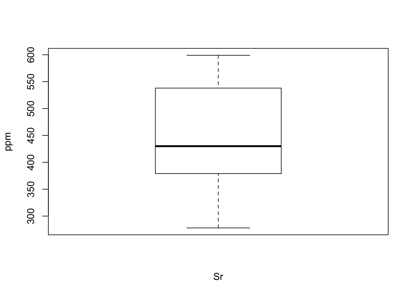
summary(sazava[,"Sr"])## Min. 1st Qu. Median Mean 3rd Qu. Max. NA's
## 278.0 392.5 430.0 443.0 537.5 599.0 2- Plot all the possible combinations of binary diagrams(a scatter plot matrix) for the following oxides: SiO2, MgO, CaO, Na2O, K2O, and P2O5.
oxides <- c("SiO2", "MgO", "CaO", "Na2O", "K2O", "P2O5")
pairs(sazava[,oxides])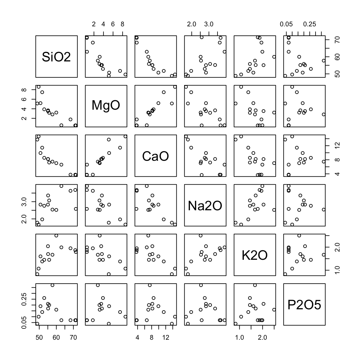
2.4. Classification and Grouping - Using Factors
Exercise 2.5. Using factors to deal with complex datasets I
- For the Sázava dataset define a factor intrusion based on the specification given in the column ‘Intrusion’ that splits the suite into three groups: basic (quartz diorites to Amp gabbros of numerous smaller bodies), Sazava (Sázava intrusion proper: mainly Amp–Bt tonalites to quartz diorites) and Pozary (Požáry trondhjemite).
data(sazava)
intrusion <- factor(sazava[,"Intrusion"])
intrusion
## [1] Sazava Sazava Sazava Sazava Sazava basic basic basic basic basic
## [11] Pozary Pozary Pozary Pozary
## Levels: basic Pozary Sazava- Display all possible values (levels)of this factor.
levels(intrusion)## [1] "basic" "Pozary" "Sazava"- Using the factor intrusion, calculate the mean SiO2 contents for each of the rock groups in the Sazava dataset.
tapply(sazava[,"SiO2"],intrusion,mean)## basic Pozary Sazava
## 51.778 68.440 55.738- Analogously,calculate the mean concentrations of Ba.
tapply(sazava[,"Ba"],intrusion,mean,na.rm=TRUE)## basic Pozary Sazava
## 676.25 1291.25 682.25Exercise 2.6. Using factors to deal with complex datasets II
- Utilizing the function summary, calculate basic statistical parameters for SiO2 distribution in each of the rock groups of the Sázava suite (factor intrusion).
data(sazava)
intrusion <- factor(sazava[,"Intrusion"])
tapply(sazava[,"SiO2"],intrusion,summary)
## $basic
## Min. 1st Qu. Median Mean 3rd Qu. Max.
## 48.84 49.63 51.72 51.78 52.90 55.80
##
## $Pozary
## Min. 1st Qu. Median Mean 3rd Qu. Max.
## 62.95 66.96 69.69 68.44 71.17 71.42
##
## $Sazava
## Min. 1st Qu. Median Mean 3rd Qu. Max.
## 50.72 55.09 55.17 55.74 57.73 59.98- What are the means for selected trace elements (Ba, Rb, Sr and Zr) in individual intrusions?
trace <- c("Rb","Sr","Ba","Zr")
aggregate(sazava[,trace],list(Rock=intrusion),mean,na.rm=TRUE)
## Rock Rb Sr Ba Zr
## 1 basic 34.5 346.25 676.25 65.75
## 2 Pozary 59.5 460.75 1291.25 157.25
## 3 Sazava 60.5 522.00 682.25 61.00- Using the function by, print basic statistical summaries for major-element oxides in each of the rock groups.
by(sazava[,7:17],list(Rock=intrusion),summary)## Rock: basic
## SiO2 TiO2 Al2O3 FeO Fe2O3
## Min. :48.84 Min. :0.340 Min. :13.34 Min. :2.740 Min. :1.47
## 1st Qu.:49.63 1st Qu.:0.670 1st Qu.:14.17 1st Qu.:5.690 1st Qu.:2.44
## Median :51.72 Median :0.760 Median :16.98 Median :6.220 Median :2.79
## Mean :51.78 Mean :0.784 Mean :16.87 Mean :5.664 Mean :2.64
## 3rd Qu.:52.90 3rd Qu.:0.800 3rd Qu.:18.23 3rd Qu.:6.430 3rd Qu.:3.22
## Max. :55.80 Max. :1.350 Max. :21.64 Max. :7.240 Max. :3.28
## MnO MgO CaO Na2O K2O
## Min. :0.130 Min. :3.160 Min. : 7.22 Min. :1.67 Min. :0.830
## 1st Qu.:0.160 1st Qu.:3.890 1st Qu.: 8.55 1st Qu.:1.78 1st Qu.:1.070
## Median :0.160 Median :5.110 Median :11.44 Median :1.97 Median :1.380
## Mean :0.174 Mean :5.644 Mean :11.12 Mean :2.25 Mean :1.236
## 3rd Qu.:0.170 3rd Qu.:7.470 3rd Qu.:13.75 3rd Qu.:2.76 3rd Qu.:1.450
## Max. :0.250 Max. :8.590 Max. :14.64 Max. :3.07 Max. :1.450
## P2O5
## Min. :0.040
## 1st Qu.:0.100
## Median :0.140
## Mean :0.148
## 3rd Qu.:0.200
## Max. :0.260
## ------------------------------------------------------------
## Rock: Pozary
## SiO2 TiO2 Al2O3 FeO Fe2O3
## Min. :62.95 Min. :0.28 Min. :15.04 Min. :1.650 Min. :0.380
## 1st Qu.:66.96 1st Qu.:0.28 1st Qu.:15.08 1st Qu.:2.002 1st Qu.:0.395
## Median :69.69 Median :0.29 Median :15.19 Median :2.120 Median :0.435
## Mean :68.44 Mean :0.29 Mean :16.36 Mean :2.075 Mean :0.480
## 3rd Qu.:71.17 3rd Qu.:0.30 3rd Qu.:16.47 3rd Qu.:2.192 3rd Qu.:0.520
## Max. :71.42 Max. :0.30 Max. :20.02 Max. :2.410 Max. :0.670
## MnO MgO CaO Na2O
## Min. :0.0400 Min. :0.520 Min. :3.670 Min. :2.580
## 1st Qu.:0.0475 1st Qu.:0.520 1st Qu.:3.730 1st Qu.:3.368
## Median :0.0500 Median :0.535 Median :3.755 Median :3.655
## Mean :0.0500 Mean :0.840 Mean :4.447 Mean :3.450
## 3rd Qu.:0.0525 3rd Qu.:0.855 3rd Qu.:4.473 3rd Qu.:3.737
## Max. :0.0600 Max. :1.770 Max. :6.610 Max. :3.910
## K2O P2O5
## Min. :1.79 Min. :0.07
## 1st Qu.:1.85 1st Qu.:0.07
## Median :1.91 Median :0.07
## Mean :1.90 Mean :0.07
## 3rd Qu.:1.96 3rd Qu.:0.07
## Max. :1.99 Max. :0.07
## ------------------------------------------------------------
## Rock: Sazava
## SiO2 TiO2 Al2O3 FeO
## Min. :50.72 Min. :0.630 Min. :16.42 Min. :5.260
## 1st Qu.:55.09 1st Qu.:0.710 1st Qu.:17.00 1st Qu.:5.430
## Median :55.17 Median :0.750 Median :17.57 Median :5.460
## Mean :55.74 Mean :0.774 Mean :17.48 Mean :5.922
## 3rd Qu.:57.73 3rd Qu.:0.830 3rd Qu.:17.59 3rd Qu.:5.810
## Max. :59.98 Max. :0.950 Max. :18.82 Max. :7.650
## Fe2O3 MnO MgO CaO Na2O
## Min. :1.000 Min. :0.120 Min. :2.82 Min. :7.04 Min. :2.520
## 1st Qu.:1.350 1st Qu.:0.150 1st Qu.:3.21 1st Qu.:7.47 1st Qu.:2.540
## Median :2.130 Median :0.160 Median :3.52 Median :8.20 Median :2.830
## Mean :1.866 Mean :0.172 Mean :3.68 Mean :8.17 Mean :2.816
## 3rd Qu.:2.190 3rd Qu.:0.190 3rd Qu.:3.67 3rd Qu.:8.22 3rd Qu.:2.830
## Max. :2.660 Max. :0.240 Max. :5.18 Max. :9.92 Max. :3.360
## K2O P2O5
## Min. :1.600 Min. :0.16
## 1st Qu.:1.670 1st Qu.:0.17
## Median :1.700 Median :0.19
## Mean :1.902 Mean :0.22
## 3rd Qu.:2.040 3rd Qu.:0.21
## Max. :2.500 Max. :0.37Excercise 2.7: Classification using factors
Classify samples in the Sázava set according to SiO2 contents (wt. %) in four groups, U (< 45), B (45–52), I (52–63) and A (> 63).
data(sazava)
silica <- cut(sazava[,"SiO2"],breaks=c(0,45,52,63,100),
              labels=c("U","B","I","A"))
silica
## [1] I I I B I I B B B I I A A A
## Levels: U B I Aacidity <- as.vector(silica)
names(acidity) <- rownames(sazava)
acidity## Sa-1 Sa-2 Sa-3 Sa-4 Sa-7 SaD-1 Gbs-1 Gbs-20 Gbs-2 Gbs-3 Po-1
## "I" "I" "I" "B" "I" "I" "B" "B" "B" "I" "I"
## Po-3 Po-4 Po-5
## "A" "A" "A"Exercise 2.8: Frequency tables
- Using the factor intrusion, count the number of analyses obtained from each of the rock groups in the Sazava dataset.
data(sazava)
intrusion <- factor(sazava[,"Intrusion"])
table(intrusion)
## intrusion
## basic Pozary Sazava
## 5 4 5- Analously, count the number of ultrabasic, basic, intermediate and acid rocks (factor silica from the previous exercise)
table(silica)## silica
## U B I A
## 0 4 7 3- Set up a frequency table showing the depencedence of silica on the rock type.
table(intrusion, silica)## silica
## intrusion U B I A
## basic 0 3 2 0
## Pozary 0 0 1 3
## Sazava 0 1 4 0Note:
Quite an amazing chapter, onward to chapter 3!
Share this post