This post is a compilation of the exercises from Chapter 3: Classical Plots from the book Geochemical Modelling of Igneous Processes - Principles and Recipes in R language by Vojtěch Janoušek, Jean Hervé Martin, Vojtěch Erban and Colin Farrow.
sink("/dev/null"); suppressPackageStartupMessages(library(GCDkit)); sink();In this chapter, I followed the examples from the book and modified the code where necessary. This includes the basic to some fundamental geochemical plots (classification and spider diagrams).
Binary Plots
Plotting Simple Binary Plots
In this exercise we focus on graphical analysis of the Sázava dataset. a) Build a binary plot SiO\(_2\)–CaO. Choose suitable ranges for the axes,label them and annotate data points by sample names. Assign the plotting symbols according to individual rock types (utilizing the pre-defined column “Symbol”).
Plot a line SiO2/CaO = 10 passing through origin [0,0].
Plot a diagram logZr – logBa and fit the data points,using the least-square linear regression, by a straight line.
sazava <- read.table("data/sazava.data",sep="\t")
par(mfrow=c(1,2))
par(mar=c(4,4,1,1))
plot(sazava[,"SiO2"],sazava[,"CaO"], cex=1.2,
     xlab=expression(SiO[2]),ylab="CaO",
     pch=sazava[,"Symbol"],xlim=c(49,75),ylim=c(0,15))
text(sazava[,"SiO2"],sazava[,"CaO"],rownames(sazava),
     pos=4,cex=0.7)
abline(0,0.1)
plot(sazava[,"Zr"],sazava[,"Ba"],xlab="Zr",ylab="Ba",
     pch=15,cex=1.5,log="xy")
lq <- lm(log10(sazava[,"Ba"]) ~ log10(sazava[,"Zr"]))
lq
##
## Call:
## lm(formula = log10(sazava[, "Ba"]) ~ log10(sazava[, "Zr"]))
##
## Coefficients:
## (Intercept) log10(sazava[, "Zr"])
## 1.1994 0.8847abline(lq,lty=2,lwd=2,col="darkgreen")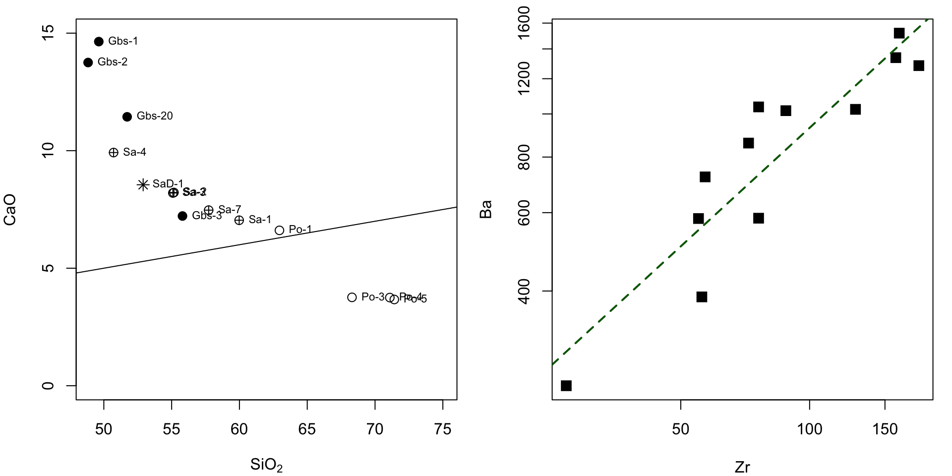
Constant Sum Effect (Closure)
The correlation in binary plots involving silica is spurious due to the constant sum effect (if one oxide increases in abundance, all others must decrease). Therefore, oxide* is introduced to represent the proportion of the relevant oxide in the non-silica portion of the rock (in wt.%):
\[oxide*=100\times \frac{oxide}{(100-SiO_2)}\]
data(sazava)
oxides <- c("TiO2","Al2O3","FeO","Fe2O3","MnO","MgO","CaO","Na2O","K2O","P2O5")

ee <- sapply(rownames(sazava),function(i){
    z<-100*sazava[i,oxides]/(100-sazava[i,"SiO2"])
    return(z)
    }
)
oxide_star<-t(ee)
par(mfrow=c(1,2))
# Panel a
plot(sazava[,"SiO2"],sazava[,"Al2O3"],col=sazava[,"Colour"],pch=sazava[,"Symbol"],cex=1.5,xlim=c(45,100),ylim=c(0,40),xaxs="i",yaxs="i",xlab=expression(SiO[2]),ylab=expression(Al[2]*O[3]))
text(82,37,cex = 1.5,
     labels = expression(Si*O[2]*"+"*Al[2]*O[3]*" > 100%"))
text(82,32,cex = 1.5,
     labels = expression("'Forbidden zone'"))
# Forbidden zone
polygon(c(100,60,100,100),c(0,40,40,0),density=10,col="gray")

# Panel b
plot(sazava[,"SiO2"],oxide_star[,"Al2O3"],col=sazava[,"Colour"],pch=sazava[,"Symbol"],cex=1.5,xlim=c(45,100),ylim=c(0,60),xaxs="i",yaxs="i",xlab=expression(SiO[2]),ylab=expression(Al[2]*O[3]*"*"))
text(70,10, cex = 1.5,
     labels = expression(Al[2]*O[3]*"* = 100 x "*frac(oxide,(100 - SiO[2]))))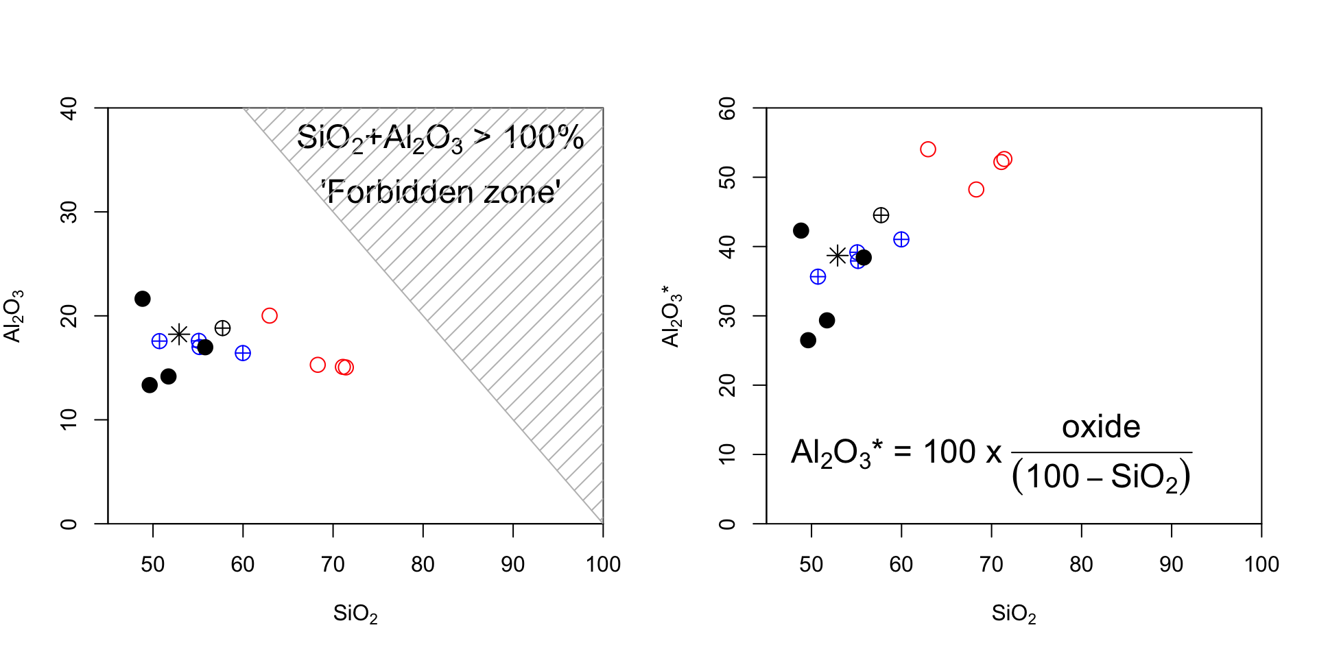
GCD solution
windows(width=10,height=5)
par(mfrow=c(1,2))
par(mar=c(4,4,1,1))
data(sazava)
accessVar("sazava")
binary("SiO2","CaO",cex=1.2)
abline(0,0.1)
binary("Zr","Ba",log="xy",pch=15,cex=1.5,col="black",fit=TRUE)
Harker Plots and Other Basic Multiple Plots
Exercise 3.2: Harker plots
Using a loop and function par(mfrow), write a short program that would plot six binary plots of SiO\(_2\) vs. major-element oxides of your choice.
data(sazava)
par(mfrow=c(2,3))
ee <- c("Al2O3","MgO","CaO","Na2O","K2O","P2O5")
for (f in ee){
plot(sazava[,"SiO2"],sazava[,f],xlab="SiO2",
ylab=f,pch=sazava[,"Symbol"],cex=1.5)
}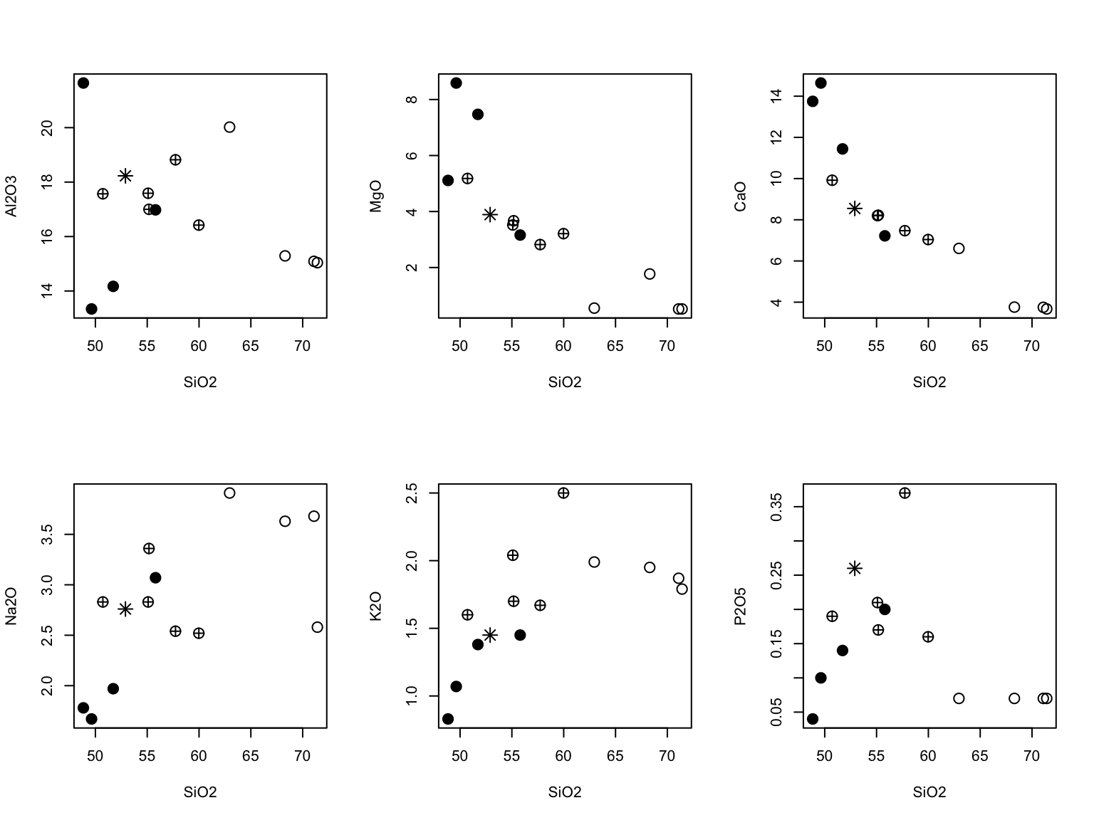 Advanced solution for nicer x-axis label
data(sazava)
par(mfrow=c(2,3))
ee <- c("Al2O3","MgO","CaO","Na2O","K2O","P2O5")
lab <- c("Al[2]*O[3]","MgO","CaO","Na[2]*O","K[2]*O","P[2]*O[5]")
for (f in 1:length(ee)){
  plot(sazava[,"SiO2"],sazava[,ee[f]],xlab=expression(SiO[2]),
       ylab=parse(text=as.expression(lab[f])),
       pch=sazava[,"Symbol"],cex=1.5)
}
GCD solution
data(sazava)
accessVar("sazava")
multiple("SiO2","Al2O3,MgO,CaO,Na2O,K2O,P2O5")
Ternary Plots
Exercise 3.3. Ternary Plots
- Design a function plotting ternary diagrams.
- Display a Ba-Rb-Sr ternary plot for the Sazava suite.
tri <- function(data,alab, blab, clab){
sums <- apply(data[,c(alab,blab,clab)],1,sum)
a <- data[,alab]/sums
b <- data[,blab]/sums
x <- 1 - a - b/2
y <- sqrt(3)*b/2
plot(x,y,xlab="",ylab="",xlim=c(0,1),
ylim=c(0,1),axes=FALSE,asp=1)
x1 <- c(0,1,.5,0)
y1 <- c(0,0,sqrt(3)/2,0)
lines(x1,y1)
text(-0.05,0,alab)
text(1.05,0,clab)
text(0.5,sqrt(3)/2+0.05,blab)
}
data(sazava)
tri(sazava,"Ba","Rb","Sr")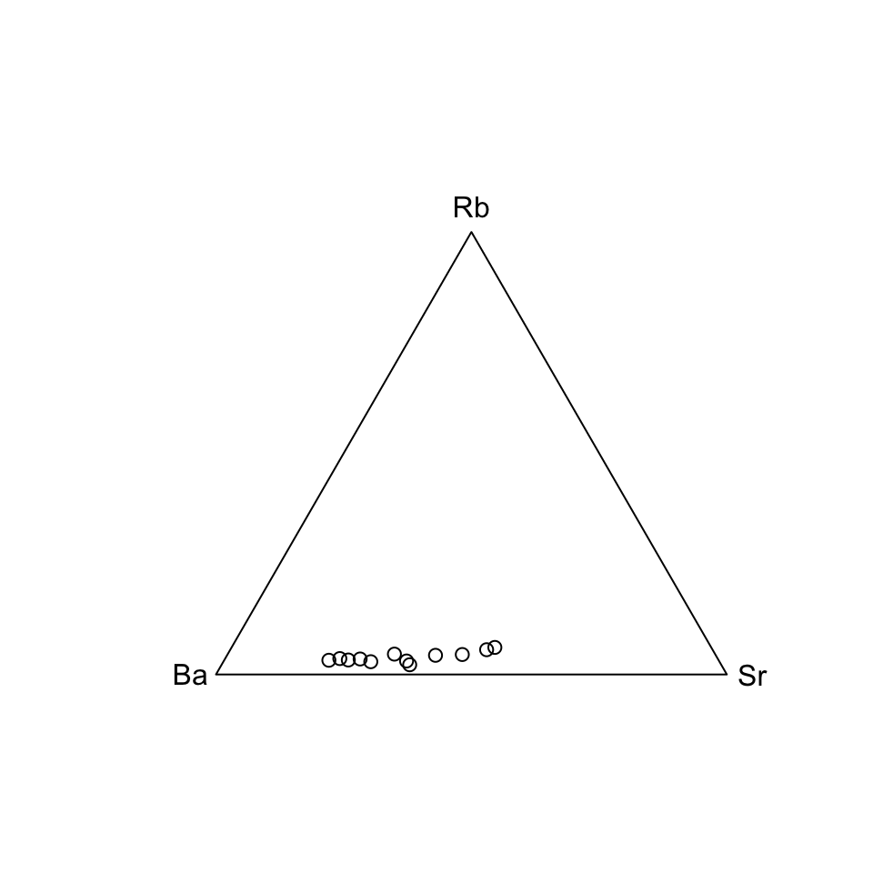 ### Geochemical plot
data(sazava)
accessVar("sazava")
plotDiagram("LarochePlut",FALSE)
classify("LarochePlut")
Spider plot
x <- read.table("data/boynton.data",sep=",")
chondrite <- as.numeric(x) # conversion to numeric vector
names(chondrite) <- names(x)

norm <- function(x,chon){
    z <- t(x[,names(chon)])/chon
    return(z)
}

data(sazava)
y <- norm(sazava,chondrite)
plot(y[,"Po-1"],type="o",log="y",axes=FALSE,xlab="",ylab="REE/chondrite",ylim=c(0.1,100),col="darkgreen")
axis(1,1:length(chondrite),labels=names(chondrite),cex.axis=0.75)
axis(2,cex.axis=0.75)
points(y[,"Po-4"],col="blue")
lines(y[,"Po-4"],col="blue")
abline(h=(10^(-1:3)),lty="dashed")
box()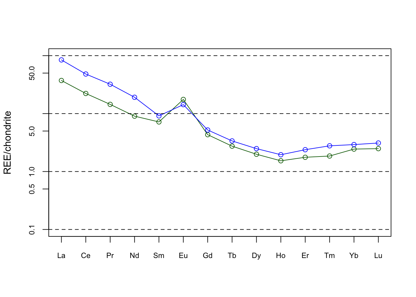
data(sazava)
accessVar("sazava")
spider(WR,"Boynton",0.1,1000,pch=labels$Symbol,col=labels$Colour)
spider(WR,"Boynton",field=TRUE,density=0.02,angle=45, col="gray",fill.col=FALSE,add=TRUE) 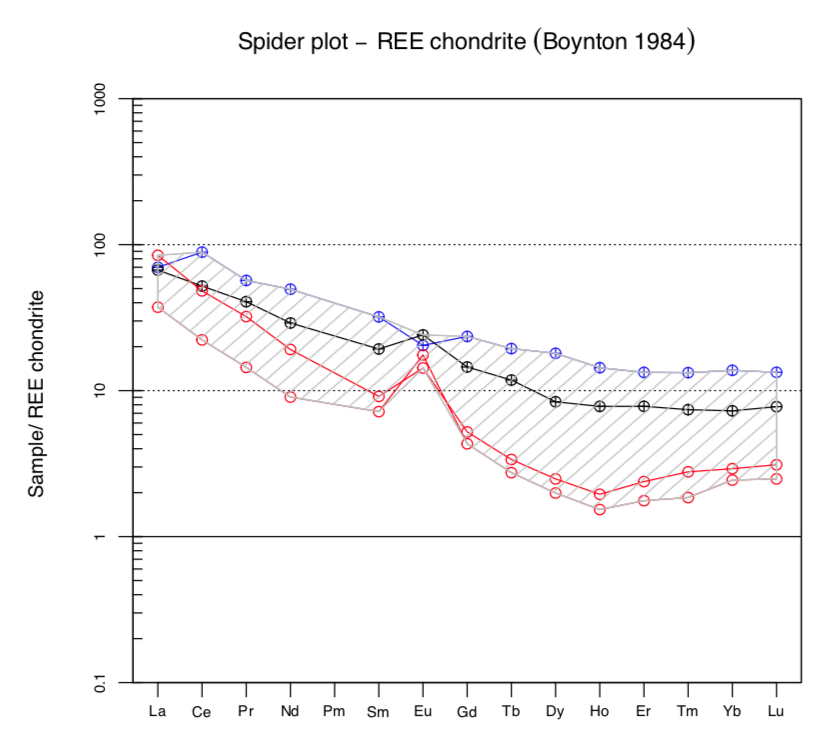
Share this post