Log-log binary plots

data(sazava)
par(mfrow=c(1,2))                       # Split screen for 2 graphs
par(mar=c(4,4,1,1))                     # Outer margins for each of the graphs

# Plot 1
plot(sazava[,"Sr"],sazava[,"Rb"],xlim=c(1,1000),ylim=c(1,1000),xlab="Sr",ylab="Rb",pch=16,col="blue",cex=1.5,xaxs="i",yaxs="i",log="")
invisible(sapply(c(seq(0.1,1,0.1),1:10),function(i)abline(0,i,lty="dashed")))

# Plot 2
plot(sazava[,"Sr"],sazava[,"Rb"],xlim=c(1,1000),ylim=c(1,1000),xlab="Sr",ylab="Rb",pch=16,col="blue",cex=1.5,xaxs="i",yaxs="i",log="xy")
invisible(sapply(c(seq(0.1,1,0.1),1:10),function(i)abline(log10(i),1,lty="dashed")))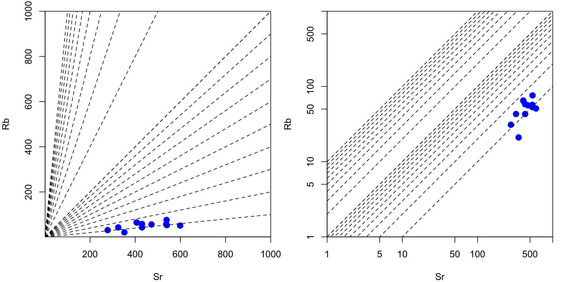

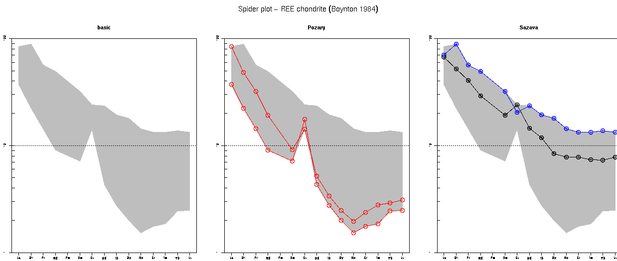
Specialized spider plots

loadData("dolerites.data")

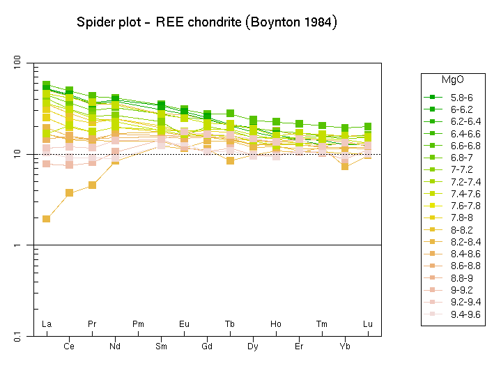
# Panel a
ee<-spider.contour("Boynton","MgO",colour.palette="terrain.colors",0.1,100,cex=1.5)

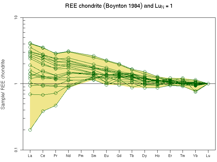
# Panel b
ee<-spider2norm(WR,"Boynton","Lu",0.1,10,pch=1,col="darkgreen",cex=1.5)
ee<-spider2norm(WR,"Boynton","Lu",field=TRUE,fill.col=TRUE,shaded.col="khaki",add=TRUE)

data(sazava)
accessVar("sazava")
groupsByLabel("Intrusion")
spider(WR,"Boynton",1,100,pch=labels$Symbol,col=labels$Colour,cex=2)
figMulti(nrow=1,ncol=3,plot.symb=TRUE)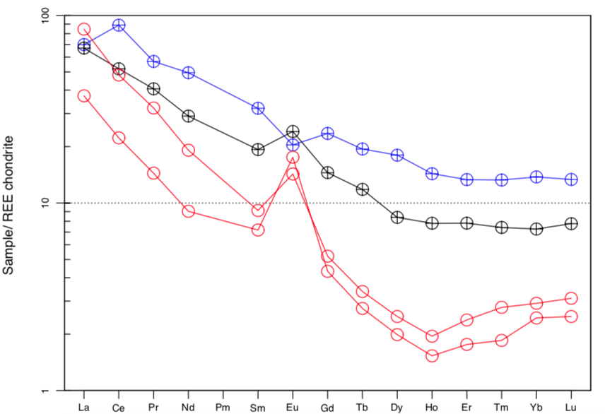

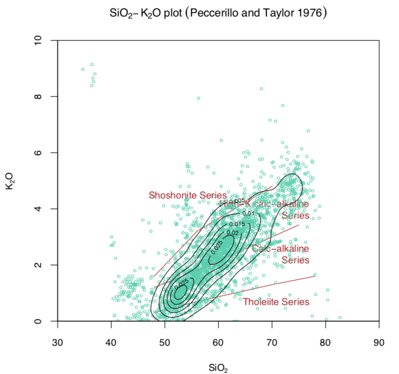
Contour plots

This is the code to call the function making contour plots. The GUI will help with further steps.

loadData("ANDEAN_ARC.csv")

# Panel a
plotDiagram("PeceTaylor",F)
figCol("aquamarine3")
addContours()

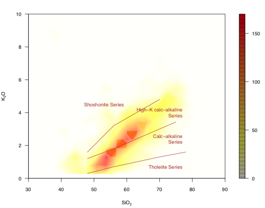
# Panel b
figRedraw()
filledContourFig()