Geochemical modelling of Ig. processes - Chapter 5: Radiogenic Isotopes

June 23, 2020 Nguyen Cong Nghia

10 minute read

Calculation of Initial Ratios or Ages
- Exercise 5.1: Initial ratios and ages
Epsilon, Delta and Gamma Values
- Exercise 5.2: Epsilon Nd values
Model Ages
Isochron Ages
- Exercise 5.5: Isochrons

This post is a compilation of the exercises from Chapter 5: Radiogenic Isotopes from the book Geochemical Modelling of Igneous Processes - Principles and Recipes in R language by Vojtěch Janoušek, Jean Hervé Martin, Vojtěch Erban and Colin Farrow.

Many of the parent-daughter dating methods are based on similar principles. The parent (radioactive) isotope decayse to ther daughter (radiogenic) isotope:

$^{87} R b \to^{87} S r$ $^{147} S m \to^{143} N d$ $^{176} L u \to^{176} H f$ $^{187} R e \to^{187} O s$

Do note that while the I ratios are measured directly with the mass spectrometer (TIMS or ICP-MS), R ratios must be calculated from elemental concentration obtained by isotope dilution, ICP-MS, XRF or other analytcal methods.

The formula based on Faure (1986)

$\frac{^{87} R b}{^{86} S r} = (\frac{C_{R b}}{C_{S r}}) [2.6939 + 0.2832 \frac{^{87} S r}{^{86} S r}]$

$\frac{^{147} S m}{^{144} N d} = (\frac{C_{S m}}{C_{N d}}) [0.53151 + 0.14252 \frac{^{143} N d}{^{144} N d}]$

Calculation of Initial Ratios or Ages

Relationship between daughter and parent ratios:

$I = R (e^{λ t} - 1)$ * I: ratio of daughter isotope to a stable, non-radiogenic isotope (e.g: $^{87} S r /^{86} S r$ , $^{143} N d /^{144} N d$ or $^{176} H f /^{177} H f$ )

R: ratio of parental isotope to the same non-radiogenic isotope in I (e.g: $^{87} R b /^{86} S r$ , $^{147} S m /^{144} N d$ or $^{176} L u /^{177} H f$ )
$λ$ : decay constant
t: time (Ma or ka)

However, due to the presence of common element present, the formula to correct the initial ratio, is modified as: $I = I_{i} + R (e^{λ t} - 1)$

$I_{i}$ : the initial ratio of common daughter-stable isotope

From this, if the age is known, the isotopic ratios can be easily ‘age-corrected’ and used in petrogenetic considerations. On the other hand, knowing the initial ratio, we can determined the age by solving for t:

$t = \frac{1}{λ} l n (\frac{I - I_{i}}{R} + 1)$

Exercise 5.1: Initial ratios and ages

The Sr–Nd isotopic study of the Central Bohemian Plutonic Complex (CBPC) (Janoušek et al. 1995) has proven a diversity of sources and processes involved in genesis of individual intrusions and suites. The file contains an excerpt from the data for several granitoid types and two country rocks.

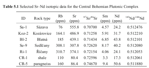
Import the data file into a matrix izo, calculate the $^{87} R b /^{86} S r$ and $^{147} S m /^{144} N d$ ratios and attach them to the matrix as the last data columns.

Design functions yielding Sr and Nd initial ratios; back-calculate these at 350 and 300 Ma ago; can you program a single function with an argument identifying the isotopic system (Sr or Nd)?

Calculate the age of the sample Koz-2 assuming that its initial ratio is 0.705.

# Part a
izo <- read.table("data/cbpizo.data", sep= "\t", check.names=F)
izo$"87Rb/86Sr" = izo$Rb/izo$Sr*(2.6939 + 0.2832*izo$`87Sr/86Sr`)
izo$"147Sm/144Nd" = izo$Sm/izo$Nd*(0.53151 + 0.14252*izo$`143Nd/144Nd`)
izo

##          Rb    Sr 87Sr/86Sr   Sm   Nd 143Nd/144Nd 87Rb/86Sr 147Sm/144Nd
## Sa-1   76.0 555.8   0.70700 4.57 24.2    0.512476 0.3957418  0.11416466
## Koz-2 164.1 486.9   0.71258 5.91 31.7    0.512210 0.9759392  0.11270205
## Bl-2  185.0 439.1   0.71434 6.85 43.8    0.512101 1.2202168  0.09453854
## Se-9  308.1 307.8   0.72620 8.17 40.2    0.512080 2.9023859  0.12285315
## Ri-1  310.7 374.1   0.72154 4.06 24.1    0.512053 2.4070655  0.10183487
## CR-1  110.0  80.4   0.72596 3.30 17.3    0.512061 3.9669665  0.11530714
## CR-5  160.0  86.4   0.74670 9.40 50.6    0.511880 5.3803064  0.11229157

#Part b
initial <- function(data, system="Sr",age){
  if (system == "Sr"){
    lambda = 1.42e-11
    I = data[,"87Sr/86Sr"]
    R = data[,"87Rb/86Sr"]
  } else if (system == "Nd"){
    lambda = 6.54e-12
    I = data[,"143Nd/144Nd"]
    R = data[,"147Sm/144Nd"]
  }
  Ii = I - R * (exp(lambda*age*10^6)-1)
  return(Ii)
}
izo$"87Sr/86Sr_i300" = initial(izo,system="Sr", age= 300)
izo$"87Sr/86Sr_i350" = initial(izo,system="Sr", age= 350)
izo$"143Nd/144Nd_i300" = initial(izo,system="Nd", age= 300)
izo$"143Nd/144Nd_i350" = initial(izo,system="Nd", age= 350)
izo[,c("87Sr/86Sr_i300","87Sr/86Sr_i350","143Nd/144Nd_i300","143Nd/144Nd_i350")]

##       87Sr/86Sr_i300 87Sr/86Sr_i350 143Nd/144Nd_i300 143Nd/144Nd_i350
## Sa-1       0.7053105      0.7050283        0.5122518        0.5122144
## Koz-2      0.7084136      0.7077175        0.5119887        0.5119517
## Bl-2       0.7091308      0.7082604        0.5119153        0.5118844
## Se-9       0.7138095      0.7117392        0.5118387        0.5117985
## Ri-1       0.7112640      0.7095471        0.5118530        0.5118196
## CR-1       0.7090247      0.7061951        0.5118345        0.5117968
## CR-5       0.7237310      0.7198933        0.5116595        0.5116227

#Part c
ini87Sr_86Sr = 0.705
lambda = 1.42e-11
age_Koz2 = 1/lambda*log((izo["Koz-2","87Sr/86Sr"]-ini87Sr_86Sr)/izo["Koz-2","87Rb/86Sr"] + 1)
age_Koz2/10^6

## [1] 544.85

An alternative solution for part b (authors’ solution):

izo <- read.table("data/cbpizo.data", sep= "\t", check.names=F)
izo$"87Rb/86Sr" = izo$Rb/izo$Sr*(2.6939 + 0.2832*izo$`87Sr/86Sr`)
izo$"147Sm/144Nd" = izo$Sm/izo$Nd*(0.53151 + 0.14252*izo$`143Nd/144Nd`)
initial <- function(data,system="Sr",age){
  # data = matrix to be recalculated
  # system = "Sr" or "Nd", age = age in Ma
  lambda <- c(1.42*10^-11,6.54*10^-12)
  names(lambda) <- c("Sr","Nd")
  R <- cbind(data[,"147Sm/144Nd"],data[,"87Rb/86Sr"])
  colnames(R) <- c("Nd","Sr")
  I <- cbind(data[,"143Nd/144Nd"],data[,"87Sr/86Sr"])
  colnames(I) <- c("Nd","Sr")
  X <- I[,system]-R[,system]*(exp(lambda[system]*
    age*10^6)-1)
return(X) 
}
izo <- cbind(izo,initial(izo,"Sr",350),
  initial(izo,"Sr",300),initial(izo,"Nd",350),
  initial(izo,"Nd",300))
colnames(izo)[9:12] <- c("87Sr/86Sr.350","87Sr/86Sr.300",
  "143Nd/144Nd.350","143Nd/144Nd.300") 
print(izo[,9:12])

##       87Sr/86Sr.350 87Sr/86Sr.300 143Nd/144Nd.350 143Nd/144Nd.300
## Sa-1      0.7050283     0.7053105       0.5122144       0.5122518
## Koz-2     0.7077175     0.7084136       0.5119517       0.5119887
## Bl-2      0.7082604     0.7091308       0.5118844       0.5119153
## Se-9      0.7117392     0.7138095       0.5117985       0.5118387
## Ri-1      0.7095471     0.7112640       0.5118196       0.5118530
## CR-1      0.7061951     0.7090247       0.5117968       0.5118345
## CR-5      0.7198933     0.7237310       0.5116227       0.5116595

Epsilon, Delta and Gamma Values

The initial Nd isotopic ratios do not differ much among inidividual rock samples, therefore they are compared to undifferentiated mantle (which is equal to chondiritic meteorites CHUR) at the time of their generation. Geochemists define the term $ϵ_{N d}$ to express this comparison:

$ϵ_{N d}^{i} = (\frac{(\frac{^{143} N d}{^{144} N d})_{i s a m p l e}}{(\frac{^{143} N d}{^{144} N d})_{i C H U R}} - 1) \times 10^{4}$ * t: intrusion age, indexes i decipher initial isotopic ratios

The present-day composition of the CHUR is $^{147} S m /^{144} N d_{C H U R} = 0.1967$ and $^{143} N d /^{144} N d_{C H U R} = 0.512638$ (Jacobsen and Wasserburg 1980) or $^{147} S m /^{144} N d_{C H U R} = 0.1960$ and $^{143} N d /^{144} N d_{C H U R} = 0.512630$ (Bouvier et al. 2008). For an overview of alternatives, as well as of error propagation, see Ickert (2013).

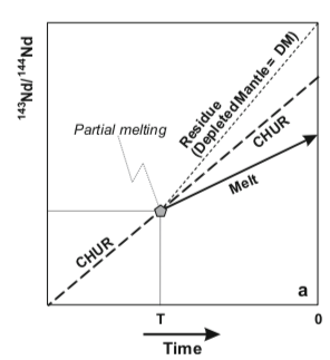
As Nd is more incompatible than Sm, partial metling of a mantle peridotite would produce melts with Sm/Nd ratios lower than the source. On the other hand, the residue would be enriched in Sm and yield a higher Sm/Nd ratio.

In contrast, the Rb-Sr system behaves in an opposite way. Rb is more incompatible than Sr in the course of mantle melting and thus the crust is characterized by high Rb/Sr, therefore, high $^{87} S r /^{86} S r$ ratios.

The geochemical-reservoir normalized compositions can be also expressed as $γ$ values, as is customary for the Re-Os system:

$γ_{O s}^{i} = (\frac{(\frac{^{187} O s}{^{188} O s})_{i s a m p l e}}{(\frac{^{187} O s}{^{188} N d})_{i C H U R}} - 1) \times 10^{2}$

The present-day mantle values are $^{187} R e /^{188} O s$ = 0.422 and $^{187} O s /^{188} O s = 0.1283$ (Walker et al. 2002).

NOTICE!

The $δ$ notation, used for stable isotopes, is analogous (just multiply by $10^{3}$ rather than $10^{2}$ ). In fact, this forms a logic system, whereby $10^{n}$ is expressed by $(n + 1)^{t h}$ letter in the Greek alphabet.

Exercise 5.2: Epsilon Nd values

Write a function returning the initial $ϵ_{N d}$ values.
Calculate these for the CBPC granitoids from the previous excercise at 350 Ma.
Plot a binary diagram of initial $^{87} S r /^{86} S r$ isotopic ratios versus initial $ϵ_{N d}$ values.

izo <- read.table("data/cbpizo.data", sep= "\t", check.names=F)
izo$"87Rb/86Sr" = izo$Rb/izo$Sr*(2.6939 + 0.2832*izo$`87Sr/86Sr`)
izo$"147Sm/144Nd" = izo$Sm/izo$Nd*(0.53151 + 0.14252*izo$`143Nd/144Nd`)

# Part a
epsNd <- function(data, age){
  RCHUR <- 0.1967; ICHUR <- 0.512638;  lambda <- 6.54e-12
  CHUR <- ICHUR - RCHUR*(exp(lambda*age*10^6)-1) #Calculate Initial CHUR ratio
  eps <- (initial(data,"Nd",age)/CHUR-1)*10^4 #Make use of "initial" function
  return(eps)
}

izo$epsilonNd_350 = round(epsNd(izo,350),2)
izo

##          Rb    Sr 87Sr/86Sr   Sm   Nd 143Nd/144Nd 87Rb/86Sr 147Sm/144Nd
## Sa-1   76.0 555.8   0.70700 4.57 24.2    0.512476 0.3957418  0.11416466
## Koz-2 164.1 486.9   0.71258 5.91 31.7    0.512210 0.9759392  0.11270205
## Bl-2  185.0 439.1   0.71434 6.85 43.8    0.512101 1.2202168  0.09453854
## Se-9  308.1 307.8   0.72620 8.17 40.2    0.512080 2.9023859  0.12285315
## Ri-1  310.7 374.1   0.72154 4.06 24.1    0.512053 2.4070655  0.10183487
## CR-1  110.0  80.4   0.72596 3.30 17.3    0.512061 3.9669665  0.11530714
## CR-5  160.0  86.4   0.74670 9.40 50.6    0.511880 5.3803064  0.11229157
##       epsilonNd_350
## Sa-1           0.53
## Koz-2         -4.60
## Bl-2          -5.91
## Se-9          -7.59
## Ri-1          -7.18
## CR-1          -7.62
## CR-5         -11.02

plot(initial(izo,age=350),epsNd(izo,350),
     xlab=expression(" "^87*Sr/""^86*Sr[i]),
     ylab=expression(epsilon[Nd]^i),
     pch=0, cex=1.5, cex.lab=1.5, cex.axis=1.5)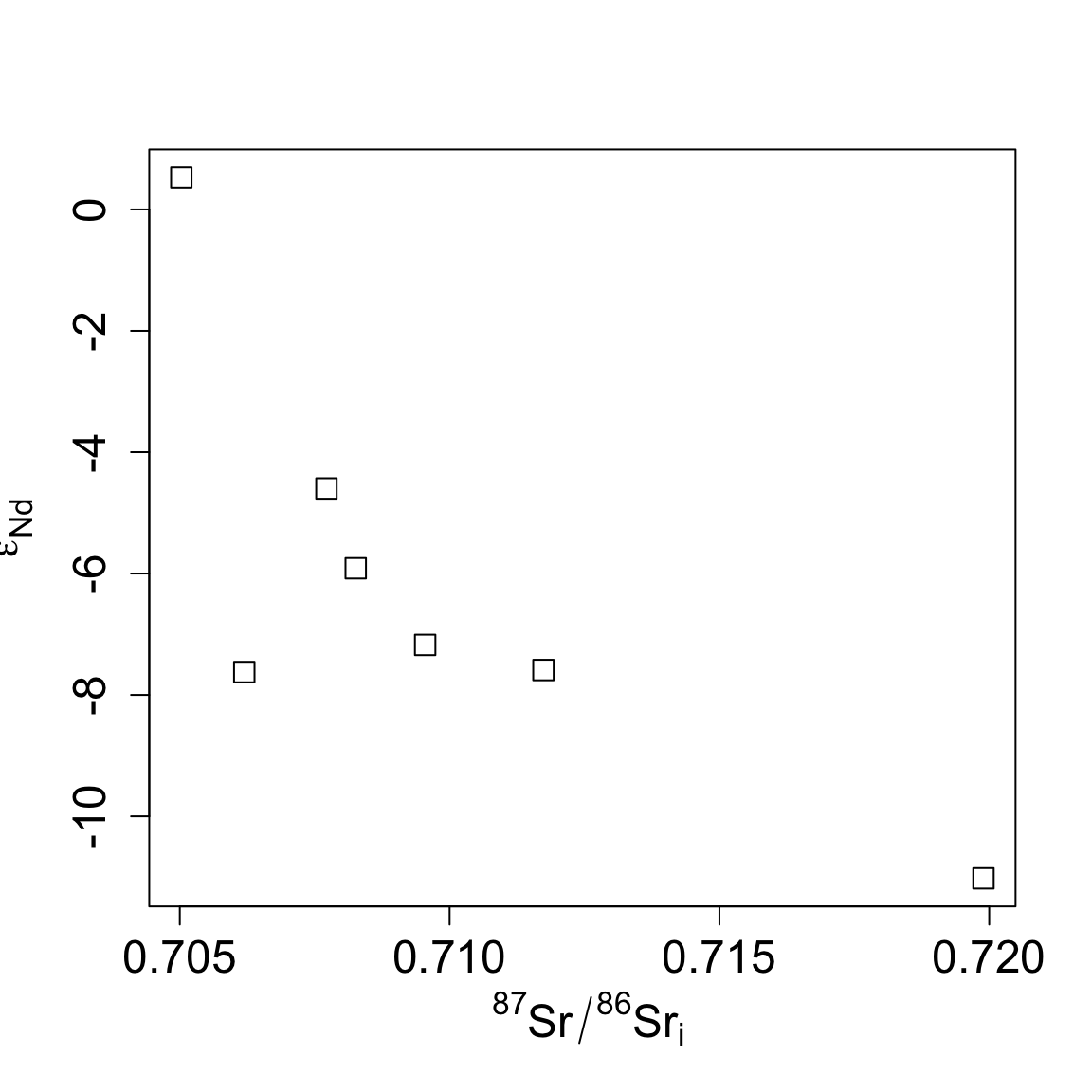

Summary of the steps to get epsilon values:

Step 1: Get the Initial CHUR
Step 2: Get the Initial ratio of $^{143} N d /^{144} N d$
Calculate the epsilon Nd, which is relative to an age.

Model Ages

The model ages represent an apparent age of extraction from a model geochemical reservoir. These include, for instance, intercepts with various mantle evolution models (often CHUR or Depleted Mantle - DM). The age is the time in the past when the given sample had the isotopic composition identical to its presumed model source reservoir. This age can be interpreted as “crust-formation ages” for a given crustal segment.

Single-stage Nd model ages

Single-stage Nd model age can be derived by setting: $I_{s a m p l e}^{T} = I_{D M}^{T}$ where DM is the appropriate model reservoir.

$I_{s a m p l e} - R_{s a m p l e} (e^{λ T} - 1) = I_{D M} - R_{D M} (e^{λ T} - 1)$ $T = \frac{1}{λ} l n (\frac{I_{s a m p l e} - I_{D M}}{R_{s a m p l e} - R_{D M}} + 1)$

The present-day composition of the DM is $^{147} S m /^{144} N d$ = 0.222 and $^{143} N d /^{144} N d$ = 0.513114

Exercise 5.3: Single-stage Nd model ages

Design a function yielding single-stage Depleted Mantle Nd model ages. Calculate these for the granitoids of the CBPC. Use the data from the previous exercises or load them from the file

DMAGE <- function(data) {
  IDM <- 0.513114
  RDM <- 0.222
  lambda <- 6.54e-12
  R <- data[,"147Sm/144Nd"]
  I <- data[,"143Nd/144Nd"]
  X <- 1/lambda*log((I-IDM)/(R-RDM)+1)/10^9
  names(X) <- rownames(data)
  return(X)
}

izo <- read.table("data/cbpizo2.data",sep="\t",check.names = F)
round(DMAGE(izo),2)

##  Sa-1 Koz-2  Bl-2  Se-9  Ri-1  CR-1  CR-5 
##  0.90  1.26  1.21  1.59  1.34  1.50  1.71

Let’s test the visualization of the solution for one sample Sa-1 with $^{143} N d /^{144} N d = 0.512476$ and $^{147} S m /^{144} N d = 0.11416466$ . From the figure, we can roughly estimate the single-stage DM model age is about 900 Ma while single-stage CHUR model age is about 300 Ma. The difference in these two values should be closer when the age is older.

t = seq(0,4600,100)
  lambda <- 6.54e-12

RCHUR <- 0.1967; ICHUR <- 0.512638 #Current CHUR ratios
CHUR <- ICHUR - RCHUR*(exp(lambda*t*10^6)-1) # Initial CHUR 

R <- 0.11416466; I <- 0.512476 #Current sample ratios
SAMP <- I - R*(exp(lambda*t*10^6)-1) #Initial Sample

RDM <- 0.222; IDM <- 0.513114 #Current DM ratios
DM <- IDM - RDM*(exp(lambda*t*10^6)-1) #Initial DM


plot(t,CHUR,type="l",xlim=c(1000,0),ylim=c(0.511,0.5133), xlab = "Age (Ma.)", ylab=expression(""^143*Nd/""^144*Nd))

lines(t,SAMP,col="red")

lines(t,DM,col="blue")

text(t[length(t)/5]-0.04,CHUR[length(CHUR)/5]+0.00009,labels = "CHUR",cex = 0.8, srt = 20)

text(t[length(t)/5]-0.04,DM[length(DM)/5]+0.00009,labels = "DM",cex = 0.8, srt = 20, col="blue")


points(t[10],DM[10])
points(t[4],CHUR[4])
text(t[10],DM[10]+0.00014,labels = expression('T'[DM]),cex=0.8)
text(t[4],CHUR[4]+0.00014,labels = expression('T'[CHUR]),cex=0.8)

points(t[1],DM[1],pch=16)
points(t[1],CHUR[1],pch=16)
points(t[1],SAMP[1],pch=16)
text(t[1],DM[1]+0.00014,labels = expression('I'[DM]),cex=0.8,)
text(t[1],CHUR[1]+0.00014,labels = expression('I'[CHUR]),cex=0.8)
text(t[1],SAMP[1]-0.00014,labels = expression('I'[sample]),cex=0.8)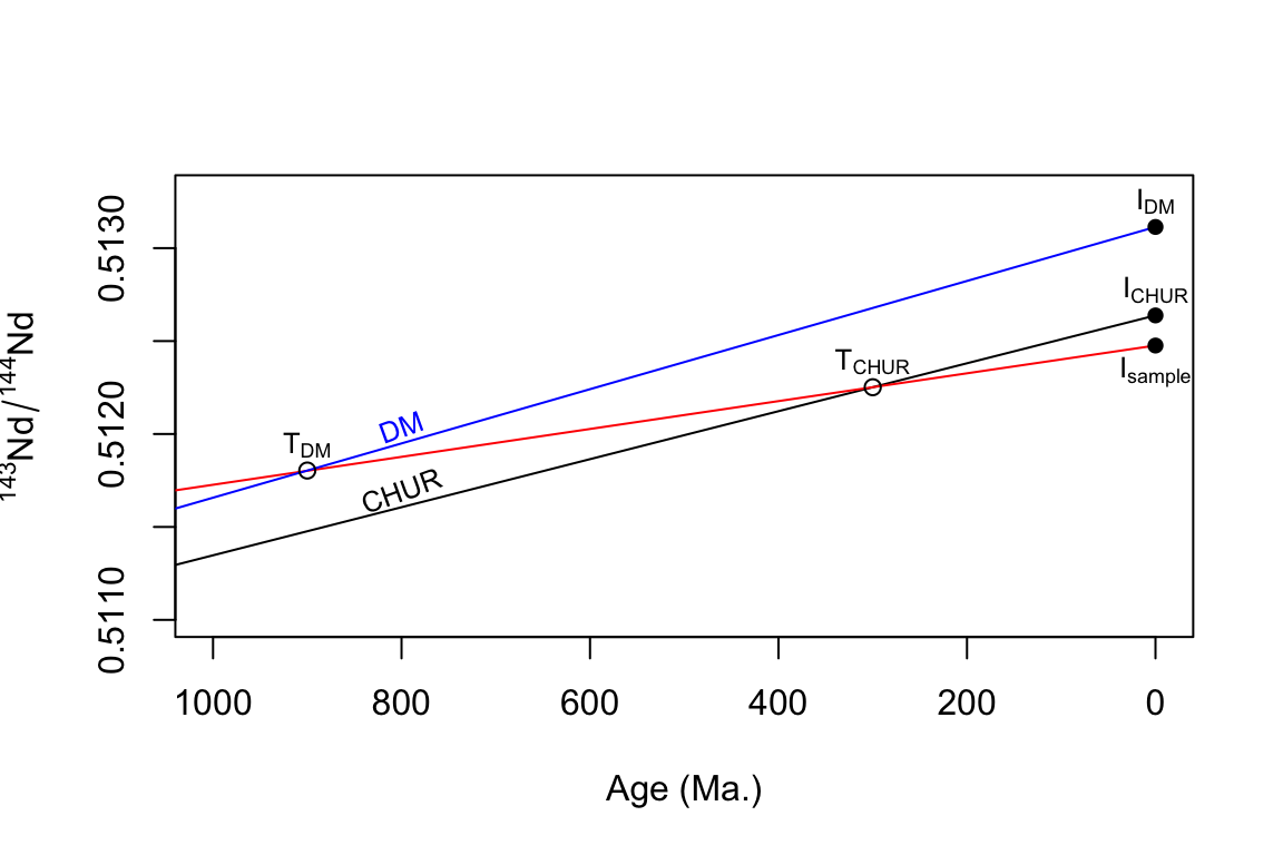

Two-stage Nd model ages

For crustally-derived rocks, the two-stage model can be used to compensate for the effects of possible second Sm/Nd fractionation (first having occurred at mantle melting) in course of the intracrustal partial melting. We have the modfied equation:

$T = \frac{1}{λ} (\frac{I_{s a m p l e}^{0} - (e^{λ t} - 1) (R_{s a m p l e}^{0} - R_{C C}^{0}) - I_{D M}^{0}}{R_{C C}^{0} - R_{D M}^{0}} + 1)$

DM: Depleted Mantle
CC: average Continental Crust
T: two-stage Nd model age; t: crystallization age of the sample

${(\frac{^{143} N d}{^{144} N d})}_{D M}^{0} = 0.513151$ ; ${(\frac{^{147} S m}{^{144} N d})}_{D M}^{0} = 0.219$ ; ${(\frac{^{147} S m}{^{144} N d})}_{C C}^{0} = 0.12$

Exercise 5.4: Two-stage Nd model ages

Design a function returning two-stage Depleted Mantle Nd model ages.
Calculate these for the granitoids of the CBPC.

DMLHAGE <- function(data,age){
  R <- data[,"147Sm/144Nd"]
  I <- data[,"143Nd/144Nd"]
  IDM <- 0.513151
  RDM <- 0.219
  RCC <- 0.12
  lambda <- 6.54e-12
  A <- I - (exp(lambda*age*1e6)-1)*(R-RCC)-IDM
  B <- RCC-RDM
  X <- 1/lambda*log(A/B+1)/10^9
  names(X) <- rownames(data)
  return(X)
}

izo <- read.table("data/cbpizo2.data",sep="\t",check.names = F)
round(DMLHAGE(izo,350),2)

##  Sa-1 Koz-2  Bl-2  Se-9  Ri-1  CR-1  CR-5 
##  1.02  1.42  1.52  1.66  1.62  1.66  1.92

Isochron Ages

When there is a cogenetic suite of whole-rock or mineral samples, the isochron ages can be determined. When consider equation $I = I_{i} + R (e^{λ t} - 1)$ with a suite of rock formed at the same age, the equation becomes:

$y = a + b x$

where a is an intercept and b is the slope of the isochron:

$b = t g α = (e^{λ t} - 1)$

which gives a formular for the isochron age:

$t = \frac{1}{λ} l n (b + 1)$

The isochrons are usually fitted using software to uilize weighted linear regression. Here are some:

Isoplot: http://www.bgc.org/isoplot_etc/isoplot.html

Ludwig, K.R., 2003. Isoplot 3.00: A geochronological toolkit for Microsoft Excel. Berkeley Geochronology Center Special Publication, 4, p.70.

Isoplotr: https://www.ucl.ac.uk/~ucfbpve/isoplotr/

Vermeesch, P., 2018. IsoplotR: A free and open toolbox for geochronology. Geoscience Frontiers, 9(5), pp.1479-1493.

UPbplot.py: https://github.com/anoda/UPbplot.py/

Sakata et al., 2017, A new approach for constraining the magnitude of initial disequilibrium in {Quaternary} zircons by coupled uranium and thorium decay series dating. Quaternary Geochronology, vol. 38, p. 1–12

Here is a simple example of making isochron without weighted linear:

Exercise 5.5: Isochrons

Read the data acari.data and plot an isochron diagam $^{87} R b /^{86} S r$ - $^{87} S r /^{86} S r$
Fit the data by straight line, calculate age and initial Sr ratio for the granite

acari <- read.table("data/acari.data", sep="\t")
colnames(acari) <- c("87Sr/86Sr","er.x","87Sr/86Sr","er.y")
plot(acari[,1],acari[,3],
     xlab=expression(""^87*Rb/""^86*Sr),
     ylab=expression(""^87*Sr/""^86*Sr),
     pch=15,cex=1.5
)
izoch <- lm(acari[,3]~acari[,1])
print(izoch)

## 
## Call:
## lm(formula = acari[, 3] ~ acari[, 1])
## 
## Coefficients:
## (Intercept)   acari[, 1]  
##     0.71171      0.02513

abline(izoch,lty="dashed")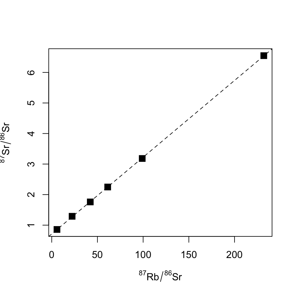

age <- 1/1.42e-11*log(izoch$coeff[2]+1)
print(age/1e6)

## acari[, 1] 
##   1747.657

post