Seeking help
First step in doing any programming is to know where to seek help. Here demonstrate how to seek help in R programming. These keywords include: help(), ?, apropos and example.
help(plot)
?plot
apropos("plot") #Commands related to "plot"
## [1] "assocplot" "barplot" "barplot.default"
## [4] "biplot" "boxplot" "boxplot.default"
## [7] "boxplot.matrix" "boxplot.stats" "cdplot"
## [10] "coplot" "fourfoldplot" "interaction.plot"
## [13] "lag.plot" "matplot" "monthplot"
## [16] "mosaicplot" "plot" "plot.default"
## [19] "plot.design" "plot.ecdf" "plot.function"
## [22] "plot.new" "plot.spec.coherency" "plot.spec.phase"
## [25] "plot.stepfun" "plot.ts" "plot.window"
## [28] "plot.xy" "preplot" "qqplot"
## [31] "recordPlot" "replayPlot" "savePlot"
## [34] "screeplot" "spineplot" "sunflowerplot"
## [37] "termplot" "ts.plot"example(plot)##
## plot> require(stats) # for lowess, rpois, rnorm
##
## plot> plot(cars)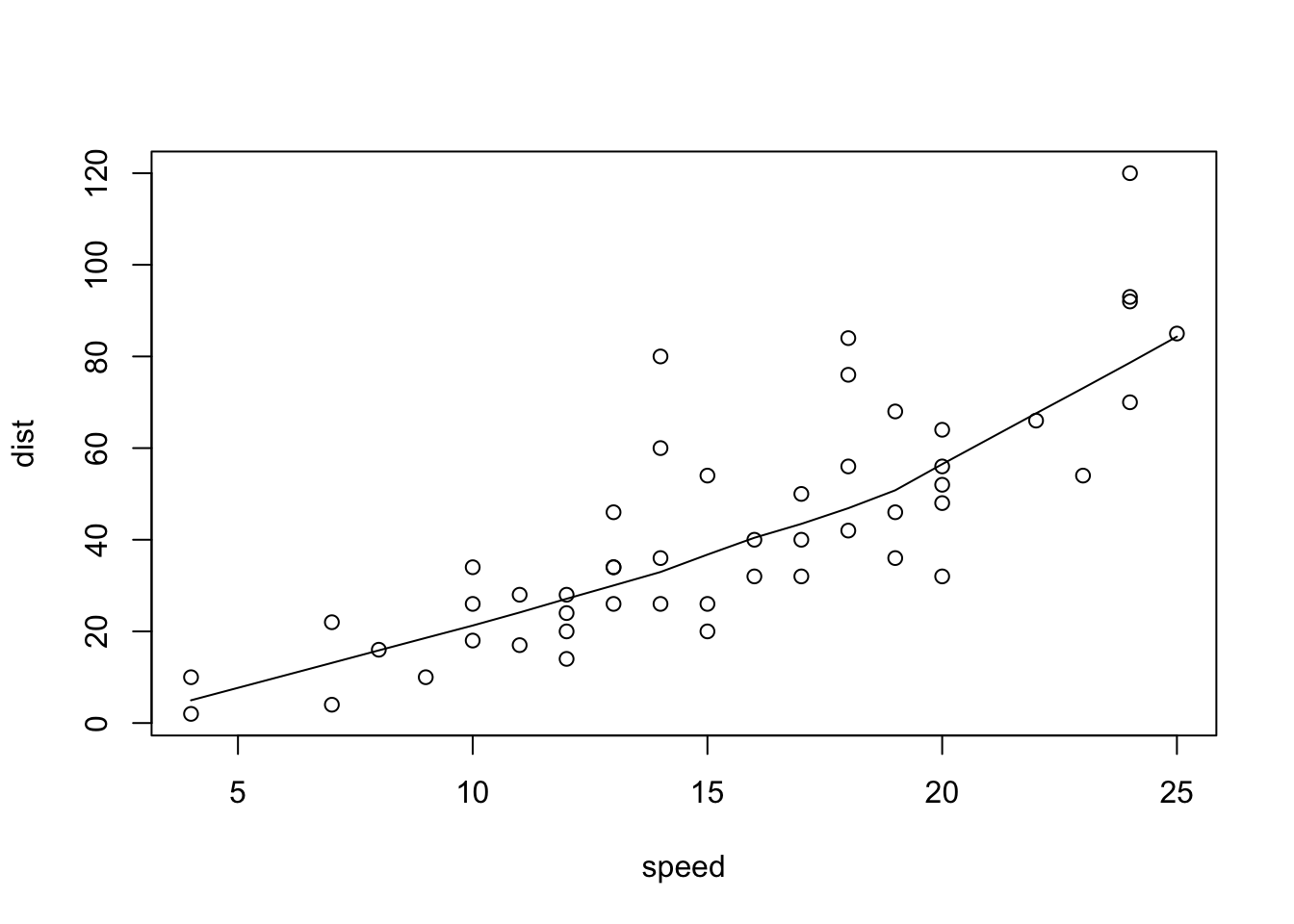
##
## plot> lines(lowess(cars))
##
## plot> plot(sin, -pi, 2*pi) # see ?plot.function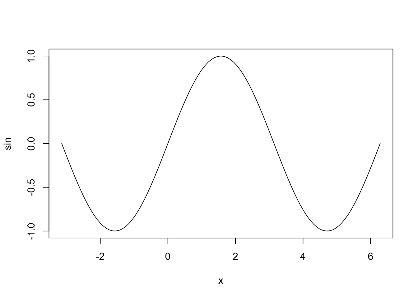
##
## plot> ## Discrete Distribution Plot:
## plot> plot(table(rpois(100, 5)), type = "h", col = "red", lwd = 10,
## plot+      main = "rpois(100, lambda = 5)")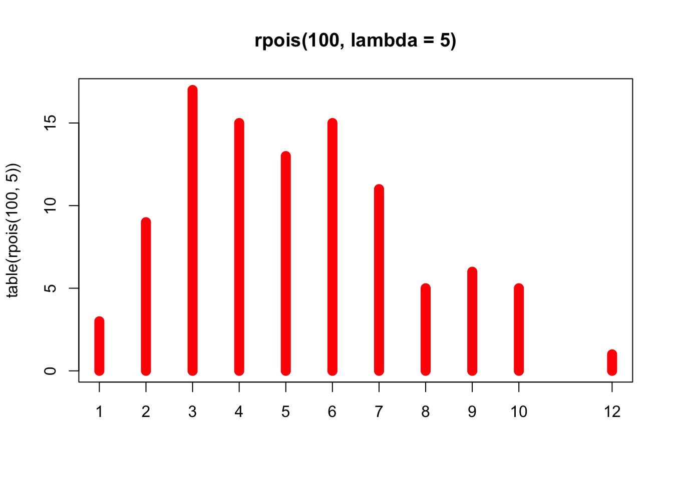
##
## plot> ## Simple quantiles/ECDF, see ecdf() {library(stats)} for a better one:
## plot> plot(x <- sort(rnorm(47)), type = "s", main = "plot(x, type = \"s\")")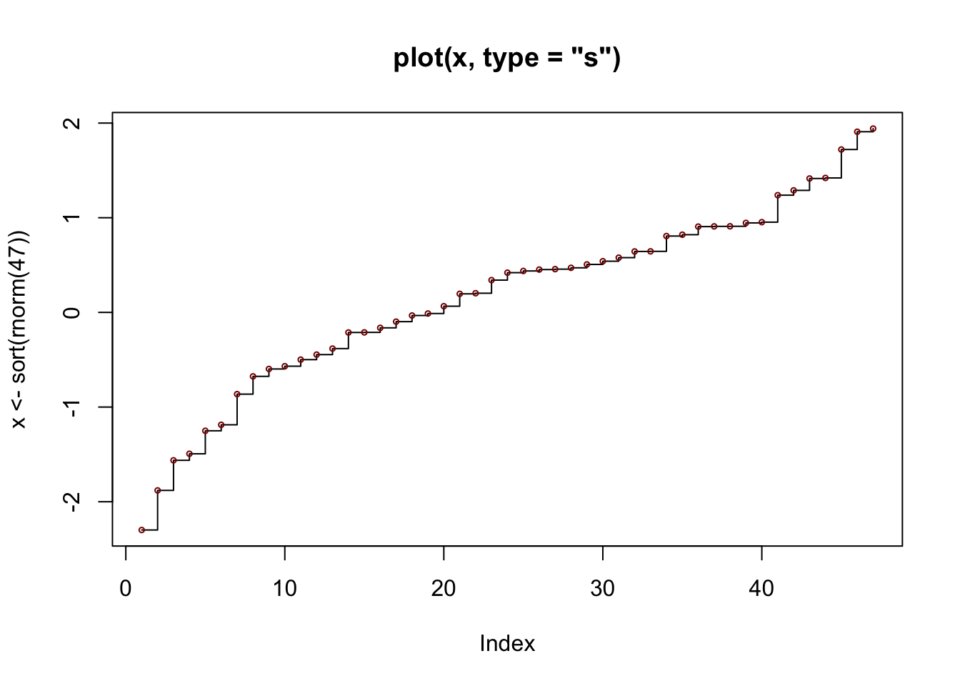
##
## plot> points(x, cex = .5, col = "dark red")
Object types
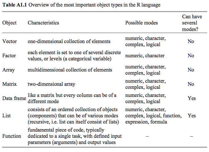
Numeric Vectors
Assignment
Assignment of several items to a vector is done using the combine function c:
x <- c(10.4, 5.6, 3.1, 6.4, 21.7)
y <- c(x,0,x)
y
## [1] 10.4 5.6 3.1 6.4 21.7 0.0 10.4 5.6 3.1 6.4 21.7Vector Arithmetic
For vectors, calculations are made using basic arithmetic operators: + - * / ^. The use of these operators for two vectors of the same length is intuitive. In other cases, the elements of the shorter vector are recycled.
x*2 #Intuitive operators of same length vectors## [1] 20.8 11.2 6.2 12.8 43.4x*c(1,2) #Multiply is recycled, i.e. *1 *2 *1 *2 *1## Warning in x * c(1, 2): longer object length is not a multiple of shorter object
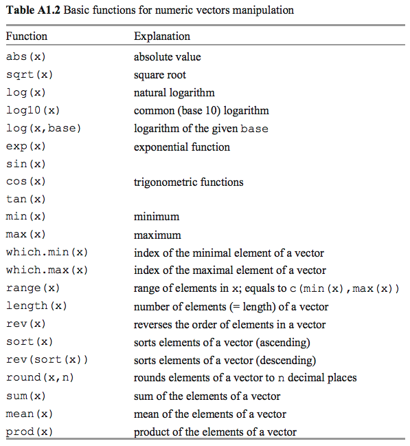
## length## [1] 10.4 11.2 3.1 12.8 21.7Functions to Manipulate Numeric Vectors
Names
Each vector may have an attribute names (the length of the vector and names must be matching)
x <- c(3,15,27)
names(x) <- c("Opx","Cpx","Pl")
x
## Opx Cpx Pl
## 3 15 27Generating Regular Sequences
Using colon, seq, rep
1:9## [1] 1 2 3 4 5 6 7 8 9seq(30,22,-2)## [1] 30 28 26 24 22x <- c(0,1)
rep(x,5)## [1] 0 1 0 1 0 1 0 1 0 1seq(0,5,length.out = 30) #linspace equivalent## [1] 0.0000000 0.1724138 0.3448276 0.5172414 0.6896552 0.8620690 1.0344828
## [8] 1.2068966 1.3793103 1.5517241 1.7241379 1.8965517 2.0689655 2.2413793
## [15] 2.4137931 2.5862069 2.7586207 2.9310345 3.1034483 3.2758621 3.4482759
## [22] 3.6206897 3.7931034 3.9655172 4.1379310 4.3103448 4.4827586 4.6551724
## [29] 4.8275862 5.0000000Character Vectors
paste("A","B","C",sep=";")## [1] "A;B;C"x <- c("A","B","C")
substring(x,1,4)## [1] "A" "B" "C"x <- c("Plagioclase","K-feldspar")
strsplit(x,"a")## [[1]]
## [1] "Pl" "giocl" "se"
##
## [[2]]
## [1] "K-feldsp" "r"Arrays, Matrices, Data Frames
Data frames are data objects with observation as columns and cases in rows, and they can contain of any mode. Matrix is a table-like object with single mode (numeric, most commonly). Arrays are generalized matrices: single mode with any number of dimensions.
x <- matrix(1:12,3,4)
x
## [,1] [,2] [,3] [,4]
## [1,] 1 4 7 10
## [2,] 2 5 8 11
## [3,] 3 6 9 12y <- matrix(1:12,3,4,byrow=TRUE)
y## [,1] [,2] [,3] [,4]
## [1,] 1 2 3 4
## [2,] 5 6 7 8
## [3,] 9 10 11 12z <- array(c(x,y), dim = c(3,4,2))
z## , , 1
##
##      [,1] [,2] [,3] [,4]
## [1,]    1    4    7   10
## [2,]    2    5    8   11
## [3,]    3    6    9   12
##
## , , 2
##
##      [,1] [,2] [,3] [,4]
## [1,]    1    2    3    4
## [2,]    5    6    7    8
## [3,]    9   10   11   12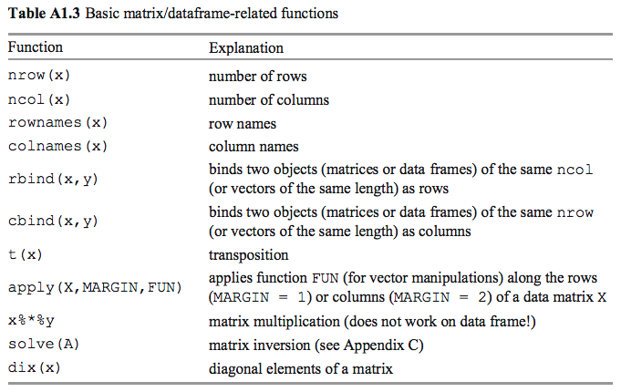
x## [,1] [,2] [,3] [,4]
## [1,] 1 4 7 10
## [2,] 2 5 8 11
## [3,] 3 6 9 12cat("Number of rows",nrow(x),"\n")## Number of rows 3cat("Number of columns", ncol(x),"\n")## Number of columns 4t(x) # transpose of x## [,1] [,2] [,3]
## [1,] 1 2 3
## [2,] 4 5 6
## [3,] 7 8 9
## [4,] 10 11 12x%*%t(x) #Multiplication of matrix x with transposition of x## [,1] [,2] [,3]
## [1,] 166 188 210
## [2,] 188 214 240
## [3,] 210 240 270apply(x,1,sum) #Sum of each row## [1] 22 26 30apply(x,2,sum) #Sum of each column## [1] 6 15 24 33Indexing/subsetting of Vectors, Arrays and Data Frames
This might be one of the most important part because manipulating and selecting data needs addition criteria. #### Vectors For more reference, see https://www.tutorialspoint.com/r/r_vectors.htm.
x <- c(1,12,15,NA,16,13,0,NA,NA)
names(x) <- c("Pl","Bt","Mu","Q","Kfs","Ky","Ol","Px","C")
x
## Pl Bt Mu Q Kfs Ky Ol Px C
## 1 12 15 NA 16 13 0 NA NALogical vector
x[x>10] #all elements > 10 or NA## Bt Mu <NA> Kfs Ky <NA> <NA>
## 12 15 NA 16 13 NA NAx[!is.na(x)] #all available elements## Pl Bt Mu Kfs Ky Ol
## 1 12 15 16 13 0Numeric vetor with positive values
x[1:5] #the first to five elements## Pl Bt Mu Q Kfs
## 1 12 15 NA 16x[c(1,5,6)] #1st, 5th and 7th elements## Pl Kfs Ky
## 1 16 13Matrices/Data Frames
Elements of a matrix are presented in the order [row, column]. If nothing is given for a row or column, it means no restriction. For more reference, see https://www.tutorialspoint.com/r/r_matrices.htm and https://www.tutorialspoint.com/r/r_data_frames.htm. For instance:
x <- matrix(1:12,3,4)
x
## [,1] [,2] [,3] [,4]
## [1,] 1 4 7 10
## [2,] 2 5 8 11
## [3,] 3 6 9 12x[1,] # all columns of the first row## [1] 1 4 7 10x[,c(1,3)] # all rows of the first and third columns## [,1] [,2]
## [1,] 1 7
## [2,] 2 8
## [3,] 3 9x[1:3,-2] # all columns apart from the 2nd of rows 1-3## [,1] [,2] [,3]
## [1,] 1 7 10
## [2,] 2 8 11
## [3,] 3 9 12If the result is a single row or column, it is automatically converted to a vector. To prevent that, one can supply drop = F:
x[1,,drop=F]## [,1] [,2] [,3] [,4]
## [1,] 1 4 7 10Manipulate matrix using index arrays:
x <- matrix(1:20,4,5)
x
## [,1] [,2] [,3] [,4] [,5]
## [1,] 1 5 9 13 17
## [2,] 2 6 10 14 18
## [3,] 3 7 11 15 19
## [4,] 4 8 12 16 20i <- matrix(c(1,2,3,3,2,1),3,2)
i## [,1] [,2]
## [1,] 1 3
## [2,] 2 2
## [3,] 3 1x[i] <- 0
x## [,1] [,2] [,3] [,4] [,5]
## [1,] 1 5 0 13 17
## [2,] 2 0 10 14 18
## [3,] 0 7 11 15 19
## [4,] 4 8 12 16 20Lists
Lists are ordered collections of other objects, which do not have to be of the same mode or type.For more references, see https://www.tutorialspoint.com/r/r_lists.htm.
x1 <- c("Luckovice","9 km E of Blatna","disused quarry")
x2 <- "melamonzonite"
x3 <- c(47.31, 1.05, 14.94, 7.01, 8.46, 10.33)
names(x3) <- c("SiO2", "TiO2", "Al2O3", "FeO", "MgO", "CaO")
luckovice <- list(ID="Gbl-4",Locality=x1,Rock=x2,major=x3)
luckovice
## $ID
## [1] "Gbl-4"
##
## $Locality
## [1] "Luckovice" "9 km E of Blatna" "disused quarry"
##
## $Rock
## [1] "melamonzonite"
##
## $major
## SiO2 TiO2 Al2O3 FeO MgO CaO
## 47.31 1.05 14.94 7.01 8.46 10.33luckovice[[1]]## [1] "Gbl-4"luckovice$Rock## [1] "melamonzonite"luckovice[[2]][3]## [1] "disused quarry"luckovice$major[c("SiO2","Al2O3")]## SiO2 Al2O3
## 47.31 14.94Factors
Factors are vector objects used for discrete classification (grouping) of components in other vectors of the same length, matrices or data frames, which is often served as categorical variables. For another reference, see https://www.tutorialspoint.com/r/r_factors.htm.
#Basic usage
x <- c("Pl","Bt","Pl","Pl","Kfs","Pl","Bt","Pl",NA)
factor(x)
## [1] Pl Bt Pl Pl Kfs Pl Bt Pl <NA>
## Levels: Bt Kfs Plordered(x,c("Pl","Kfs","Bt"))## [1] Pl Bt Pl Pl Kfs Pl Bt Pl <NA>
## Levels: Pl < Kfs < BtConversion of numeric vectors to factors
In some cases, we want to divide the total range of a numeric vector x into a certain number of discrete groups and code the values in x accroding to the rank they fall in.
numericVector <- runif(10, min = 1, max = 256 )
numericVector
## [1] 200.87228 181.25822 177.50095 254.34912 130.34155 75.24619 69.16914
## [8] 239.49859 80.69252 240.40641cut(numericVector, 3)## [1] (193,255] (131,193] (131,193] (193,255] (69,131] (69,131] (69,131]
## [8] (193,255] (69,131] (193,255]
## Levels: (69,131] (131,193] (193,255]cut(numericVector, 3, labels = c("low","med","high"))## [1] high med med high low low low high low high
## Levels: low med highcut(numericVector,breaks = c(1,100,200,256), labels = c("l","m","h"))## [1] h m m h m l l h l h
## Levels: l m htable(…) to counts the number of occurences of the givel level within the factor
vt_cut <- cut(numericVector,breaks = c(1,100,200,256), labels = c("l","m","h"))
table(vt_cut)
## vt_cut
## l m h
## 3 3 4tapply(x,INDEX,FUN,…):Apply a function to each cell of a ragged array, that is to each (non-empty) group of values given by a unique combination of the levels of certain factors. See https://www.rdocumentation.org/packages/base/versions/3.6.2/topics/tapply.
statef <- c("tas", "sa",  "qld", "nsw", "nsw", "nt",  "wa",  "wa",  "qld", "vic", "nsw", "vic", "qld", "qld", "sa",  "tas",  "sa",  "nt",  "wa",  "vic", "qld", "nsw", "nsw", "wa",  "sa",  "act", "nsw", "vic", "vic", "act")
incomes <- c(60, 49, 40, 61, 64, 60, 59, 54, 62, 69, 70, 42, 56, 61, 61, 61, 58, 51, 48, 65, 49, 49, 41, 48, 52, 46, 59, 46, 58, 43)

(incmeans <- tapply(incomes, statef, sum))
## act nsw nt qld sa tas vic wa
## 89 344 111 268 220 121 280 209aggregate(x,by,FUN,..): Splits the data into subsets, computes summary statistics for each, and returns the result in a convenient form. See https://www.rdocumentation.org/packages/stats/versions/3.6.2/topics/aggregate
data("ChickWeight")
aggregate(ChickWeight$weight,  by=list(chkID = ChickWeight$Diet), FUN=mean)
## chkID x
## 1 1 102.6455
## 2 2 122.6167
## 3 3 142.9500
## 4 4 135.2627
Share this post