Obtaining and Annotating Binary Plots

sink("/dev/null"); suppressPackageStartupMessages(library(GCDkit)); sink();

data(sazava)
plot(sazava[,"SiO2"],sazava[,"Ba"],xlab=expression(SiO[2]),
     cex=1.5,ylab="Ba",pc=16,main="Sazava",xlim=c(45,75))
abline(h=seq(0,1500,500),lty="dotted",col="gray")
abline(v=seq(40,80,10),lty="dotted",col="gray")
text(sazava[,"SiO2"],sazava[,"Ba"],rownames(sazava),pos=4,col="red")
ee <- lm(sazava[,"Ba"] ~ sazava[,"SiO2"])
ee

## 
## Call:
## lm(formula = sazava[, "Ba"] ~ sazava[, "SiO2"])
## 
## Coefficients:
##      (Intercept)  sazava[, "SiO2"]  
##         -1680.45             43.67

abline(ee,lwd=2,lty="dashed",col="blue")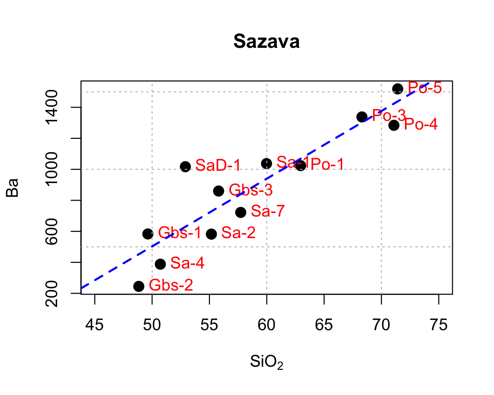

summary(ee)

## 
## Call:
## lm(formula = sazava[, "Ba"] ~ sazava[, "SiO2"])
## 
## Residuals:
##     Min      1Q  Median      3Q     Max 
## -207.22 -141.43   -4.17   96.79  387.49 
## 
## Coefficients:
##                   Estimate Std. Error t value  Pr(>|t|)    
## (Intercept)      -1680.452    386.483  -4.348   0.00145 ** 
## sazava[, "SiO2"]    43.667      6.526   6.691 0.0000542 ***
## ---
## Signif. codes:  0 '***' 0.001 '**' 0.01 '*' 0.05 '.' 0.1 ' ' 1
## 
## Residual standard error: 175.8 on 10 degrees of freedom
##   (2 observations deleted due to missingness)
## Multiple R-squared:  0.8174, Adjusted R-squared:  0.7992 
## F-statistic: 44.77 on 1 and 10 DF,  p-value: 0.00005422

data(sazava)
plot(sazava[,"Rb"],sazava[,"Sr"],xlab="Rb (ppm)",
     ylab="Sr (ppm)",pch=sazava[,"Symbol"],cex=2,
     xlim=c(0,70),ylim=c(0,650),xaxs="i",yaxs="i")
abline(0,5,col="red",lwd=1.5,lty="dashed")
curve(x^2,add=TRUE,col="blue",lwd=1.5,lty="dotted",from=0,to=25)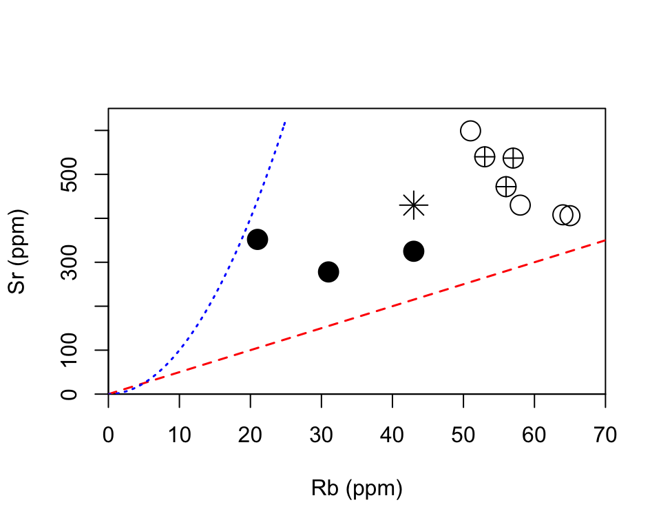

Additional High-level Plotting Functions

data(sazava)
oxides <- c("MgO","CaO","Na2O","K2O")
boxplot(sazava[,oxides],col=c("khaki","gray","red","blue"))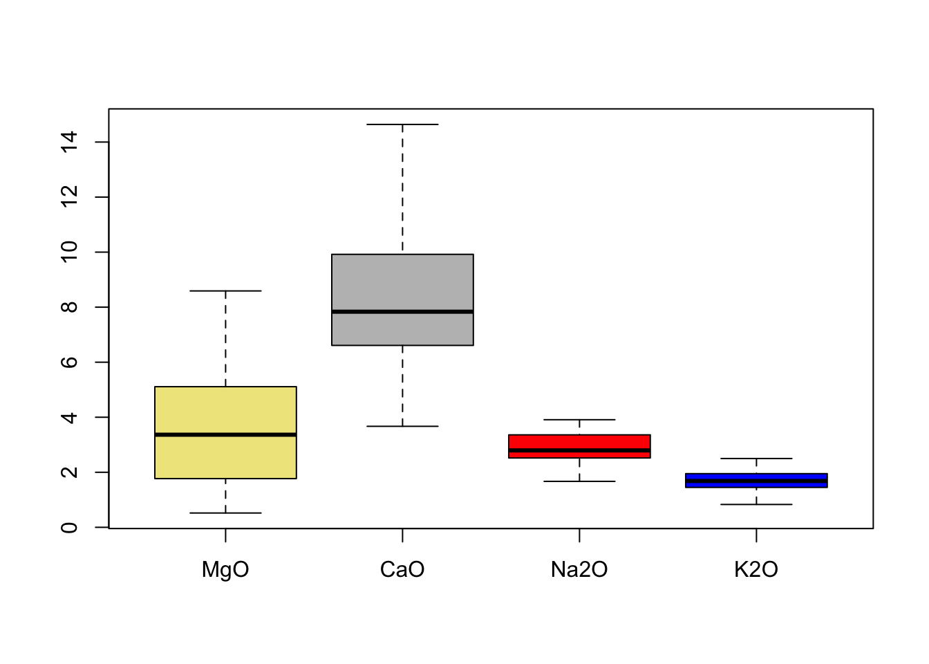

hist(sazava[,"Sr"],xlab="Sr",ylab="frequency",
     xlim=c(100,700),col="darkred",density=5, 
     angle=45, main = "Histogram of Sr")
box()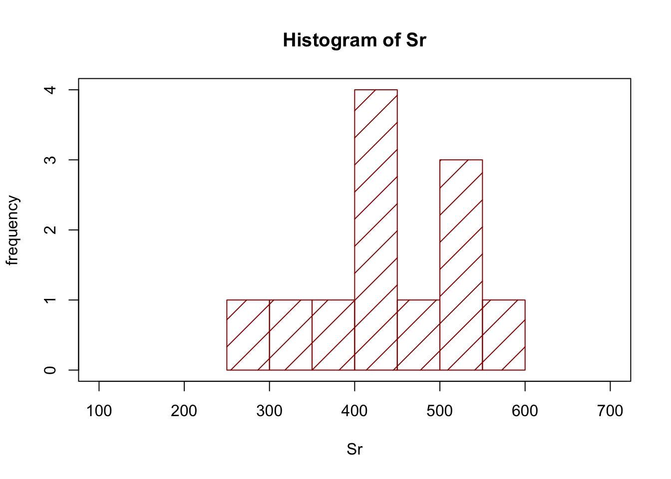

data(volcano)
contour(volcano, col="blue")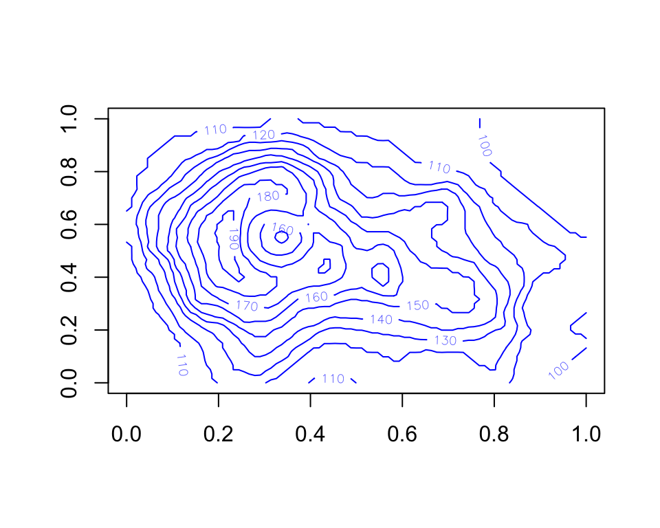

filled.contour(volcano,color.palette = terrain.colors,asp=1)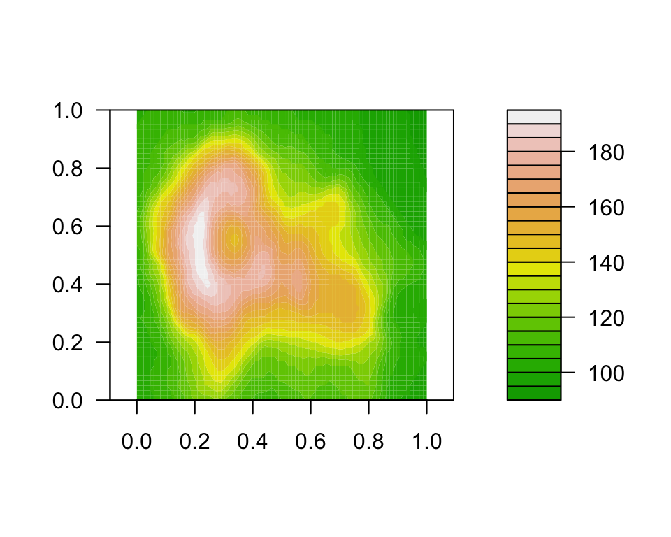

Creating Custom Layouts and Axes

plot(1,1,xlim=c(0,3),ylim=c(-1,1),axes=FALSE,
     xlab="custom X",ylab="custom Y",type="n")
axis(1,0:3,c("A","B","C","D"))
axis(2,-1:1,c("I","II","III"))
box()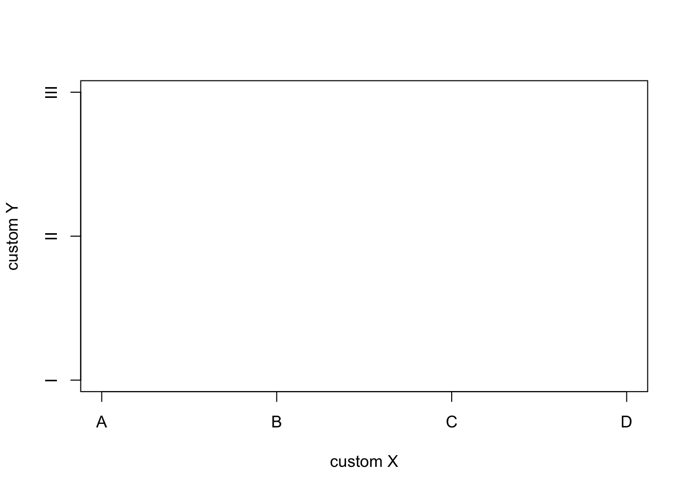

Different expression and parse text

expression(SiO[2])

## expression(SiO[2])

x <- "SiO[2]"
parse(text=as.expression(x))

## expression(SiO[2])

Exporting Graphs from R and Graphical Devices

# Create my_data
my_data <- mtcars
# Print the first 6 rows
head(my_data, 6)

##                    mpg cyl disp  hp drat    wt  qsec vs am gear carb
## Mazda RX4         21.0   6  160 110 3.90 2.620 16.46  0  1    4    4
## Mazda RX4 Wag     21.0   6  160 110 3.90 2.875 17.02  0  1    4    4
## Datsun 710        22.8   4  108  93 3.85 2.320 18.61  1  1    4    1
## Hornet 4 Drive    21.4   6  258 110 3.08 3.215 19.44  1  0    3    1
## Hornet Sportabout 18.7   8  360 175 3.15 3.440 17.02  0  0    3    2
## Valiant           18.1   6  225 105 2.76 3.460 20.22  1  0    3    1

# 1. Open a pdf file
pdf("rplot.pdf") 
# 2. Create a plot
plot(x = my_data$wt, y = my_data$mpg,
     pch = 16, frame = FALSE,
     xlab = "wt", ylab = "mpg", col = "#2E9FDF")
# Close the pdf file
dev.off() 

## quartz_off_screen 
##                 2